SpreadBounds
where , is the sorted absolute differences from a random disjoint pairing, , , and is the randomized sign-test cutoff for .
Robust bounds on with specified coverage.
Input
- — input sample of measurements, where , requires sparity(x)
- — probability that true spread falls outside bounds in the long run
Output
- Value interval bounding
- Unit same unit as
Notes
- Note disjoint-pair sign-test inversion; randomized cutoff matches requested misrate exactly under weak continuity; conservative with ties
Properties
- Shift invariance
- Scale equivariance
- Non-negativity where
- Monotonicity in misrate smaller produces wider bounds
Example
SpreadBounds([1..30], 10^(-3))returns bounds containingSpread = 9- Bounds fail to cover true spread with probability
provides distribution-free bounds on the estimate. It uses disjoint pairs and an exact sign-test inversion, which guarantees coverage regardless of the underlying distribution. Set to control how often the bounds might fail to contain the true spread: use for everyday analysis or for critical decisions. The cutoff is clamped so that , ensuring the lower and upper order statistics remain within the sorted differences.
Minimum sample size the sign test on pairs has minimum achievable misrate :
| 22 | 30 | 36 | 42 |
See also: for comparing Spread against practical thresholds with automatic verdict generation.
Algorithm
The estimator constructs distribution-free bounds on by inverting a sign test on disjoint pairs.
Given a sample , the algorithm proceeds as follows:
-
Random disjoint pairing Randomly pair the observations into disjoint pairs. If is odd, one observation is discarded. The randomization ensures that the pairing does not depend on the data ordering.
-
Absolute differences For each pair , compute the absolute difference . Under the sparity assumption, these absolute differences are exchangeable.
-
Sort Sort the differences to obtain .
-
SignMargin cutoff Compute (see SignMargin). This determines how many extreme order statistics to exclude from each tail.
-
Order statistic selection Return where and . Clamping ensures the indices remain within .
The key insight is that disjoint pairs provide independence under the symmetry assumption. Under weak symmetry around the true spread, each absolute difference is equally likely to exceed or fall below the population spread. This makes the count of differences exceeding the spread a variable, enabling exact coverage control via the sign test.
The randomized cutoff from matches the requested misrate exactly under weak continuity. With tied values, the bounds become conservative (actual coverage exceeds ).
using Pragmastat.Algorithms;
using Pragmastat.Functions;
using Pragmastat.Exceptions;
using Pragmastat.Internal;
using Pragmastat.Randomization;

namespace Pragmastat.Estimators;

/// <summary>
/// Distribution-free bounds for Spread using disjoint pairs with sign-test inversion.
/// Randomizes the cutoff between adjacent ranks to match the requested misrate.
/// Requires misrate >= 2^(1 - floor(n/2)).
/// </summary>
public class SpreadBoundsEstimator : IOneSampleBoundsEstimator
{
  public static readonly SpreadBoundsEstimator Instance = new();

  public Bounds Estimate(Sample x, Probability misrate)
  {
    return Estimate(x, misrate, null);
  }

  public Bounds Estimate(Sample x, Probability misrate, string? seed)
  {
    Assertion.NonWeighted("x", x);

    if (double.IsNaN(misrate) || misrate < 0 || misrate > 1)
      throw AssumptionException.Domain(Subject.Misrate);

    int n = x.Size;
    int m = n / 2;
    double minMisrate = MinAchievableMisrate.OneSample(m);
    if (misrate < minMisrate)
      throw AssumptionException.Domain(Subject.Misrate);

    if (x.Size < 2)
      throw AssumptionException.Sparity(Subject.X);
    if (FastSpread.Estimate(x.SortedValues, isSorted: true) <= 0)
      throw AssumptionException.Sparity(Subject.X);

    var rng = seed == null ? new Rng() : new Rng(seed);

    int margin = SignMargin.Instance.CalcRandomized(m, misrate, rng);
    int halfMargin = margin / 2;
    int maxHalfMargin = (m - 1) / 2;
    if (halfMargin > maxHalfMargin)
      halfMargin = maxHalfMargin;

    int kLeft = halfMargin + 1;
    int kRight = m - halfMargin;

    int[] indices = Enumerable.Range(0, n).ToArray();
    var shuffled = rng.Shuffle(indices);
    var diffs = new double[m];
    for (int i = 0; i < m; i++)
    {
      int a = shuffled[2 * i];
      int b = shuffled[2 * i + 1];
      diffs[i] = Math.Abs(x.Values[a] - x.Values[b]);
    }
    Array.Sort(diffs);

    double lower = diffs[kLeft - 1];
    double upper = diffs[kRight - 1];

    return new Bounds(lower, upper, x.Unit);
  }
}
Notes
targets the population spread with distribution-free coverage. This note records the approaches we discussed and tried, why most of them fail, and which theoretical limits force the final design. Here distribution-free means the stated misrate bound holds for all distributions of , not just for a parametric family or under smoothness assumptions.
Setup and notation
Let be i.i.d. real-valued observations. Let and let be a random disjoint pairing of indices independent of the values. Define
for , and let be their order statistics.
Let be the distribution of and let be any median of . The target parameter is .
Valid pivot and exact coverage
Assume weak continuity of (no ties), so . Then the sign count (the number of indices with ) has distribution . For any integer ,
Therefore the interval has coverage for all distributions of . This is the core distribution-free pivot used by .
If has atoms (ties), then for any median . The binomial pivot becomes conservative: the same interval still covers with probability at least , but exact matching of a requested misrate is impossible.
Approaches that look reasonable but fail
All pairwise differences as if independent. Construct absolute differences and apply a sign-test or binomial confidence interval as if those values were i.i.d. This ignores strong dependence between pairs, so coverage can be arbitrarily wrong. Correcting for dependence would require the joint law of all pairwise differences, which depends on the unknown distribution and is not distribution-free.
U-statistic inequalities for the median. Hoeffding-type bounds give distribution-free confidence bands for U-statistics, but for a median of pairwise differences they are extremely conservative. Intervals frequently collapse to almost , which is unusable in practice. Asymptotic U-quantile results require smoothness and density assumptions, so they are not distribution-free.
Deterministic pairing based on order or sorting. Pairing consecutive elements in the given order is value-independent, but it is not permutation-invariant: changing the input order changes the result. If the order is adversarial (or structured), coverage can deviate arbitrarily. Pairing after sorting (or pairing extremes) is value-dependent, so the distribution-free pivot no longer applies.
Choose the best pairing based on the data. Searching many pairings and picking the tightest interval is data-dependent. The selection event depends on the observed values, so coverage is not unconditional. Coverage can become arbitrarily low.
Bootstrap, asymptotic normality, or variance estimation. These are not distribution-free and can be anti-conservative for heavy tails or small samples. Studentization helps asymptotically but still depends on distributional regularity (density, smoothness, finite moments).
Mid-p or continuity-corrected binomial intervals. These reduce discreteness but do not guarantee the nominal misrate even for the binomial model itself, so the distribution-free guarantee is lost.
Deterministic disjoint pairs: why it is conservative
With disjoint pairs, the pivot is valid, but the binomial CDF is discrete. The achievable misrates form a grid
. If the requested misrate falls between grid points, a deterministic method must round down, which is conservative by design. The minimum achievable misrate is .
Deterministic interpolation between neighboring order statistics would use value distances instead of ranks, making coverage distribution-dependent and invalidating the distribution-free guarantee. As grows, the grid becomes finer (step size is ), so deterministic rounding converges asymptotically, but exact matching remains impossible for any finite .
Working approach: randomized cutoff
The final design keeps disjoint pairs but randomizes the cutoff between adjacent grid points. Let . Define and . Let be the largest integer such that and let . Choose with probability
and otherwise. This makes the tail probability exactly .
Randomization affects only the cutoff and is independent of data values, so the distribution-free property is preserved.
Theoretical limits
- Distribution-free + deterministic + exact misrate is impossible for finite . The pivot statistic is integer-valued, so the coverage function takes only finitely many values. Exact matching requires randomization.
- Exact matching for all distributions is impossible because ties break the binomial pivot. Under weak continuity (no ties), randomized cutoffs achieve exact misrate; with atoms, coverage is only guaranteed to be conservative.
- Deterministic exact misrate is possible only with extra assumptions (parametric family, smooth density at the target, known variance), which violates distribution-free guarantees.
- Any method that treats all pairwise differences as independent is invalid because dependence destroys the binomial pivot.
- Any data-dependent choice of pairing or cutoff breaks unconditional coverage and can make the method arbitrarily anti-conservative.
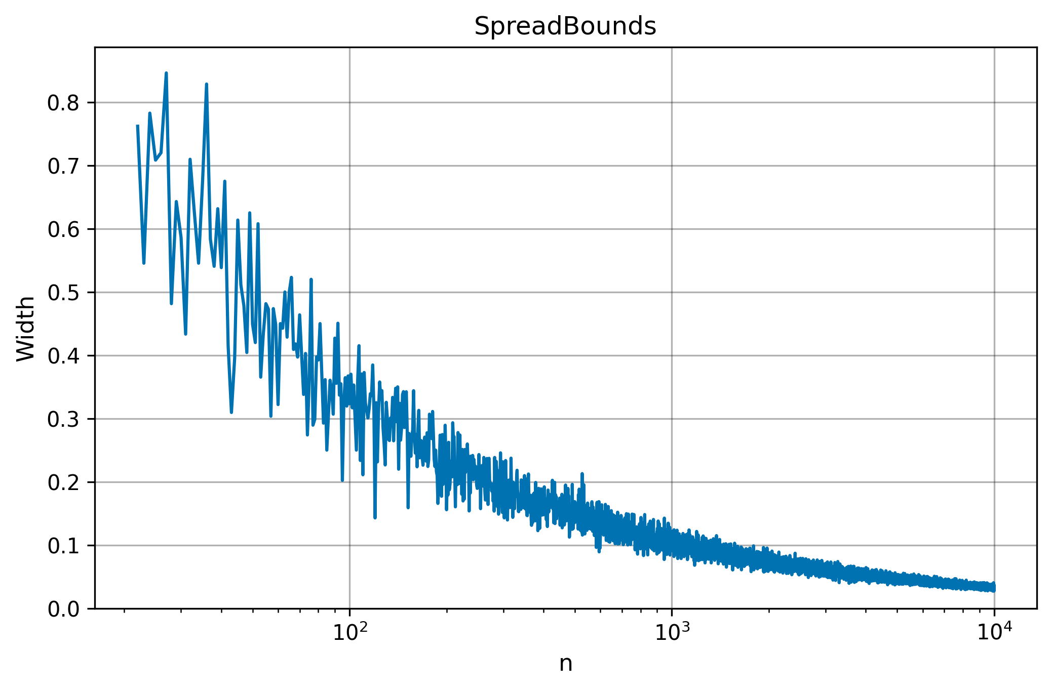
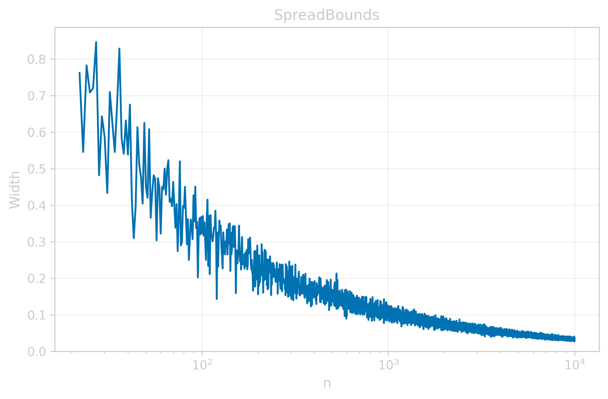
Width Convergence
The table below shows how narrows as grows, for ( evenly spaced points on ) and . Dashes indicate too small to achieve the target misrate.
| N | Width |
|---|---|
| 2 | — |
| 3 | — |
| 4 | — |
| 5 | — |
| 10 | — |
| 20 | — |
| 30 | 0.5862 |
| 40 | 0.5385 |
| 50 | 0.4490 |
| 100 | 0.3232 |
| 200 | 0.1558 |
| 300 | 0.2241 |
| 400 | 0.1479 |
| 500 | 0.1663 |
| 1000 | 0.0981 |
| 10000 | 0.0326 |
Tests
Let . Draw a value-independent random disjoint pairing of the sample, compute for , and sort ascending.
Let be the largest integer such that . If the target lies between two adjacent CDF steps, is randomized between and to match the requested misrate. Define and .
Return .
The test suite contains 43 test cases (3 demo + 4 natural + 4 property + 7 edge + 3 additive + 2 uniform + 5 misrate + 5 conservatism + 8 unsorted + 2 error). Since returns bounds rather than a point estimate, tests validate that bounds are well-formed and satisfy equivariance properties under a fixed seed. Each test case output is a JSON object with lower and upper fields representing the interval bounds. Because pairing and cutoff selection are randomized, tests fix seed to keep outputs deterministic.
Demo examples from manual introduction, validating basic bounds:
demo-1: , bounds containingdemo-2: , stricter fixture misrate, wider boundsdemo-3: , looser fixture misrate
These cases illustrate how tighter misrates produce wider bounds and how sample size affects bound width.
Natural sequences 4 tests:
natural-10:natural-15:natural-20:natural-30:
Property validation () 4 tests:
property-identity: , bounds must containproperty-location-shift: (= identity + 10), bounds must equal identity bounds (shift invariance)property-scale-2x: (= 2 identity), bounds must be 2 identity bounds (scale equivariance)property-scale-neg: (= identity), bounds must equal identity bounds ( scaling)
Edge cases boundary conditions and extreme scenarios (7 tests):
edge-small-non-trivial: (small but non-trivial bounds)edge-large-misrate: (permissive bounds)edge-duplicates-mixed: (partial ties)edge-wide-range: (extreme value range)edge-negative: (negative values)edge-large-n: (large sample, tighter sign-test bounds)edge-n2: (minimum sample size, only the maximal achievable misrate is valid)
Additive distribution (reference fixture misrates) 3 tests with :
additive-20:additive-30:additive-50:
Uniform distribution (reference fixture misrates) 2 tests with :
uniform-20:uniform-50:
Misrate variation () 5 tests with varying fixture misrates:
These tests validate monotonicity: smaller misrates produce wider bounds.
Conservatism tests (loose achievable fixture misrates) 5 tests unique to :
conservatism-12: , sign-test bounds are wide relative toconservatism-15:conservatism-20:conservatism-30:conservatism-50:
These tests document how discreteness-driven conservatism decreases with increasing sample size. For small , bounds may span a large part of the pairwise-difference range. For large , bounds tighten to a practical interval around .
Unsorted tests verify stable behavior on non-sorted inputs (8 tests):
unsorted-reverse-10:unsorted-reverse-15: ,unsorted-shuffle-10: shuffledunsorted-shuffle-15: shuffled,unsorted-negative-5: negative values unsortedunsorted-mixed-signs-5: mixed signs unsortedunsorted-duplicates: , unsorted with duplicatesunsorted-wide-range: , unsorted wide range
These tests validate that produces sensible bounds for arbitrary input order under a fixed seed.
Error cases inputs that violate assumptions (2 tests):
error-empty-x: — empty array violates validityerror-constant-x: () — constant sample violates sparity ()
Note: has a minimum misrate constraint. The sign-test inversion requires .