CenterBounds
where (pairwise averages, sorted) for , , , and
Robust bounds on with specified coverage.
Input
- — input sample of measurements, where
- — probability that true center falls outside bounds in the long run
Output
- Value — interval bounding
- Unit — same unit as
Notes
- Also known as — Wilcoxon signed-rank confidence interval for Hodges-Lehmann pseudomedian
- Note — assumes weak symmetry and weak continuity; exact for , Edgeworth approximation for
Properties
- Shift equivariance
- Scale equivariance
Example
CenterBounds([1..10], 10^(-3))returns bounds containingCenter = 5.5- Bounds fail to cover true center with probability
provides not just the estimated center but also the uncertainty of that estimate. The function returns an interval of plausible center values given the data. Set to control how often the bounds might fail to contain the true center: use for everyday analysis or for critical decisions where errors are costly. These bounds require weak symmetry but no specific distributional form. If the bounds exclude some reference value, that suggests the true center differs reliably from that value.
See also: for comparing Center against practical thresholds with automatic verdict generation.
Algorithm
uses two components: SignedRankMargin to determine which order statistics to select, and a fast quantile algorithm to compute them.
The estimator computes the median of all pairwise averages for . For , we need not just the median but specific order statistics: the -th smallest pairwise average for bounds computation. Given a sample of size , there are such pairwise averages.
A naive approach would materialize all pairwise averages, sort them, and extract the desired quantile. With , this creates approximately 50 million values, requiring quadratic memory and time. The fast algorithm avoids materializing the pairs entirely.
The algorithm exploits the sorted structure of the implicit pairwise average matrix. After sorting the input to obtain , the pairwise averages form a symmetric matrix where both rows and columns are sorted. Instead of searching through indices, the algorithm searches through values. It maintains a search interval , initialized to (the range of all possible pairwise averages). At each iteration, it asks: How many pairwise averages are at most this threshold? Based on the count, it narrows the search interval. For finding the -th smallest pairwise average: if , the target is at or below the threshold and the search continues in the lower half; if , the target is above the threshold and the search continues in the upper half.
The key operation is counting pairwise averages at or below a threshold . For each , we need to count how many satisfy , equivalently . Because the array is sorted, a single pass through the array suffices. For each , a pointer tracks the largest index where . As increases, increases, so the threshold decreases, meaning can only decrease (or stay the same). This two-pointer technique ensures each element is visited at most twice, making the counting operation regardless of the threshold value.
Binary search converges to an approximate value, but bounds require exact pairwise averages. After the search converges, the algorithm identifies candidate exact values near the approximate threshold, then selects the one at the correct rank. The candidate generation examines positions near the boundary: for each row , it finds the values where the pairwise average crosses the threshold, collecting the actual pairwise average values. Sorting these candidates and verifying ranks ensures the exact quantile is returned.
needs two quantiles: and . The algorithm computes each independently using the same technique. For symmetric bounds around the center, the lower and upper ranks are and .
The algorithm achieves time complexity for sorting, plus for binary search where is the value range precision. Memory usage is for the sorted array plus for candidate generation. This is dramatically more efficient than the naive approach. For , the fast algorithm completes in milliseconds versus minutes for the naive approach.
The algorithm uses relative tolerance for convergence: . The floor of 1 prevents degenerate tolerance when bounds are near zero. This ensures stable behavior across different scales of input data. For candidate generation near the threshold, small tolerances prevent missing exact values due to floating-point imprecision.
using System.Diagnostics;

namespace Pragmastat.Algorithms;

/// <summary>
/// Efficiently computes quantiles from all pairwise averages (x[i] + x[j]) / 2 for i ≤ j.
/// Uses binary search with counting function to avoid materializing all N(N+1)/2 pairs.
/// </summary>
internal static class FastCenterQuantiles
{
  private static bool IsSorted(IReadOnlyList<double> list)
  {
    for (int i = 1; i < list.Count; i++)
      if (list[i] < list[i - 1])
        return false;
    return true;
  }
  /// <summary>
  /// Relative epsilon for floating-point comparisons in binary search convergence.
  /// </summary>
  private const double RelativeEpsilon = 1e-14;
  /// <summary>
  /// Compute specified quantile from pairwise averages.
  /// </summary>
  /// <param name="sorted">Sorted input array.</param>
  /// <param name="k">1-based rank of the desired quantile.</param>
  /// <returns>The k-th smallest pairwise average.</returns>
  public static double Quantile(IReadOnlyList<double> sorted, long k)
  {
    Debug.Assert(
      IsSorted(sorted),
      "FastCenterQuantiles.Quantile: input must be sorted");
    int n = sorted.Count;
    if (n == 0)
      throw new ArgumentException("Input cannot be empty", nameof(sorted));

    long totalPairs = (long)n * (n + 1) / 2;
    if (k < 1 || k > totalPairs)
      throw new ArgumentOutOfRangeException(nameof(k), $"k must be in range [1, {totalPairs}]");

    if (n == 1)
      return sorted[0];

    return FindExactQuantile(sorted, k);
  }

  /// <summary>
  /// Compute both lower and upper bounds from pairwise averages.
  /// </summary>
  /// <param name="sorted">Sorted input array.</param>
  /// <param name="marginLo">Rank of lower bound (1-based).</param>
  /// <param name="marginHi">Rank of upper bound (1-based).</param>
  /// <returns>Lower and upper quantiles.</returns>
  public static (double Lo, double Hi) Bounds(IReadOnlyList<double> sorted, long marginLo, long marginHi)
  {
    Debug.Assert(
      IsSorted(sorted),
      "FastCenterQuantiles.Bounds: input must be sorted");
    int n = sorted.Count;
    if (n == 0)
      throw new ArgumentException("Input cannot be empty", nameof(sorted));

    long totalPairs = (long)n * (n + 1) / 2;

    marginLo = Max(1, Min(marginLo, totalPairs));
    marginHi = Max(1, Min(marginHi, totalPairs));

    double lo = FindExactQuantile(sorted, marginLo);
    double hi = FindExactQuantile(sorted, marginHi);

    return (Min(lo, hi), Max(lo, hi));
  }

  /// <summary>
  /// Count pairwise averages ≤ target value.
  /// </summary>
  private static long CountPairsLessOrEqual(IReadOnlyList<double> sorted, double target)
  {
    int n = sorted.Count;
    long count = 0;
    // j is not reset: as i increases, threshold decreases monotonically
    int j = n - 1;

    for (int i = 0; i < n; i++)
    {
      double threshold = 2 * target - sorted[i];

      while (j >= 0 && sorted[j] > threshold)
        j--;

      if (j >= i)
        count += j - i + 1;
    }

    return count;
  }

  /// <summary>
  /// Find exact k-th pairwise average using selection algorithm.
  /// </summary>
  private static double FindExactQuantile(IReadOnlyList<double> sorted, long k)
  {
    int n = sorted.Count;
    long totalPairs = (long)n * (n + 1) / 2;

    if (n == 1)
      return sorted[0];

    if (k == 1)
      return sorted[0];

    if (k == totalPairs)
      return sorted[n - 1];

    double lo = sorted[0];
    double hi = sorted[n - 1];
    const double eps = RelativeEpsilon;

    var candidates = new List<double>(n);

    while (hi - lo > eps * Max(1.0, Max(Abs(lo), Abs(hi))))
    {
      double mid = (lo + hi) / 2;
      long countLessOrEqual = CountPairsLessOrEqual(sorted, mid);

      if (countLessOrEqual >= k)
        hi = mid;
      else
        lo = mid;
    }

    double target = (lo + hi) / 2;

    for (int i = 0; i < n; i++)
    {
      double threshold = 2 * target - sorted[i];

      int left = i;
      int right = n;

      while (left < right)
      {
        int m = (left + right) / 2;
        if (sorted[m] < threshold - eps)
          left = m + 1;
        else
          right = m;
      }

      if (left < n && left >= i && Abs(sorted[left] - threshold) < eps * Max(1.0, Abs(threshold)))
        candidates.Add((sorted[i] + sorted[left]) / 2);

      if (left > i)
      {
        double avgBefore = (sorted[i] + sorted[left - 1]) / 2;
        if (avgBefore <= target + eps)
          candidates.Add(avgBefore);
      }
    }

    if (candidates.Count == 0)
      return target;

    candidates.Sort();

    foreach (double candidate in candidates)
    {
      long countAtCandidate = CountPairsLessOrEqual(sorted, candidate);
      if (countAtCandidate >= k)
        return candidate;
    }

    return target;
  }
}
Notes
On Bootstrap for Center Bounds
A natural question arises: can bootstrap resampling improve coverage for asymmetric distributions where the weak symmetry assumption fails?
The idea is appealing. The signed-rank approach computes bounds from order statistics of Walsh averages using a margin derived from the Wilcoxon distribution, which assumes symmetric deviations from the center. Bootstrap makes no symmetry assumption: resample the data with replacement, compute on each resample, and take quantiles of the bootstrap distribution as bounds. This should yield valid bounds regardless of distributional shape.
This manual deliberately does not provide a bootstrap-based alternative to . The reasons are both computational and statistical.
Computational cost
computes bounds in time: a single pass through the Walsh averages guided by the signed-rank margin. No resampling, no iteration.
A bootstrap version requires resamples (typically for stable tail quantiles), each computing on the resample. itself costs via the fast selection algorithm on the implicit pairwise matrix. The total cost becomes per call — roughly slower than the signed-rank approach.
For , each call to operates on Walsh averages. The bootstrap recomputes this times. The computation is not deep — it is merely wasteful. For , there are Walsh averages per resample, and resamples produce selection operations per bounds call. In a simulation study that evaluates bounds across many samples, this cost becomes prohibitive.
Statistical quality
Bootstrap bounds are nominal, not exact. The percentile method has well-documented undercoverage for small samples: requesting high confidence (for example, ) often yields materially higher actual misrate for . This is inherent to the bootstrap percentile method — the quantile estimates from resamples are biased toward the sample and underrepresent tail behavior. Refined methods (BCa, bootstrap-) partially address this but add complexity and still provide only asymptotic guarantees.
Meanwhile, provides exact distribution-free coverage under symmetry. When the requested misrate matches an achievable signed-rank level, the method attains that level exactly. A bootstrap method targeting the same nominal misrate can materially undercover on small samples. The exact method is simultaneously faster and more accurate.
Behavior under asymmetry
Under asymmetric distributions, the signed-rank margin is no longer calibrated: the Wilcoxon distribution assumes symmetric deviations, and asymmetry shifts the actual distribution of comparison counts.
However, the coverage degradation is gradual, not catastrophic. Mild asymmetry produces mild coverage drift. The bounds remain meaningful — they still bracket the pseudomedian using order statistics of the Walsh averages — but the actual misrate differs from the requested value.
This is the same situation as bootstrap, which also provides only approximate coverage. The practical difference is that the signed-rank approach achieves this approximate coverage in time, while bootstrap achieves comparable approximate coverage in time.
Why not both?
One might argue for providing both methods: the signed-rank approach as default, and a bootstrap variant for cases where symmetry is severely violated.
This creates a misleading choice. If the bootstrap method offered substantially better coverage under asymmetry, the complexity would be justified. But for the distributions practitioners encounter (, , and other moderate asymmetries), the coverage difference between the two approaches is small relative to the cost difference. For extreme asymmetries where the signed-rank coverage genuinely breaks down, the sign test provides an alternative foundation for median bounds (see On Misrate Efficiency of MedianBounds), but its efficiency convergence makes it impractical for moderate sample sizes.
The toolkit therefore provides as the single bounds estimator. The weak symmetry assumption means the method performs well under approximate symmetry and degrades gracefully under moderate asymmetry. There is no useful middle ground that justifies a computational penalty for marginally different approximate coverage.
On Misrate Efficiency of MedianBounds
This note analyzes , a bounds estimator for the population median based on the sign test, and explains why pragmastat omits it in favor of .
Definition
where is the largest integer satisfying and . The interval brackets the population median using order statistics, with controlling the probability that the true median falls outside the bounds.
requires no symmetry assumption — only weak continuity — making it applicable to arbitrarily skewed distributions. This is its principal advantage over , which assumes weak symmetry.
Sign test foundation
The method is equivalent to inverting the sign test. Under weak continuity, each observation independently falls above or below the true median with probability . The number of observations below the median follows , and the order statistics and form a confidence interval whose coverage is determined exactly by the binomial CDF.
Because the binomial CDF is a step function, the achievable misrate values form a discrete set. The algorithm rounds down to the nearest achievable level, inevitably wasting part of the requested misrate budget. This note derives the resulting efficiency loss and its convergence rate.
Achievable misrate levels
The achievable misrate values for sample size are:
The algorithm selects the largest satisfying . The efficiency measures how much of the requested budget is used. Efficiency means the bounds are as tight as the misrate allows; means half the budget is wasted, producing unnecessarily wide bounds.
Spacing between consecutive levels
The gap between consecutive achievable misrates is:
For a target , the relevant index satisfies . By the normal approximation to the binomial, , the binomial CDF near this index changes by approximately:
where is the corresponding standard normal quantile and is the standard normal density. This spacing governs how coarsely the achievable misrates are distributed near the target.
Expected efficiency
The requested falls at a uniformly random position within a gap of width . On average, the algorithm wastes , giving expected efficiency:
Define the misrate-dependent constant:
Then the expected efficiency has the form:
The convergence rate is : efficiency improves as the square root of sample size.
The constant increases for smaller misrates, meaning tighter error tolerances require proportionally larger samples for efficient bounds. This is one reason why the finer signed-rank resolution matters most when practitioners request or stricter.
Comparison with CenterBounds
uses the signed-rank statistic with range . Under the null hypothesis, has variance . The CDF spacing at the relevant quantile is:
The expected efficiency for is therefore:
This converges at rate — three polynomial orders faster than . The difference arises because the signed-rank distribution has discrete levels compared to the binomials levels, providing fundamentally finer resolution.
Why pragmastat omits MedianBounds
The efficiency loss of is not an implementation artifact. It reflects a structural limitation of the sign test: using only the signs of discards magnitude information, leaving only binary observations to determine coverage. The signed-rank test used by exploits both signs and ranks, producing comparison outcomes and correspondingly finer misrate resolution.
For applications requiring tight misrate control on the median, large samples () are needed to ensure efficient use of the misrate budget. For smaller samples, the bounds remain valid but conservative: the actual misrate is guaranteed to not exceed the requested value, even though it may be substantially below it.
with its convergence achieves near-continuous misrate control even for moderate , at the cost of requiring weak symmetry. For the distributions practitioners typically encounter, this tradeoff favors as the single bounds estimator in the toolkit. When symmetry is severely violated, the coverage drift of is gradual — mild asymmetry produces mild drift — making it a robust default without the efficiency penalty inherent to the sign test approach.
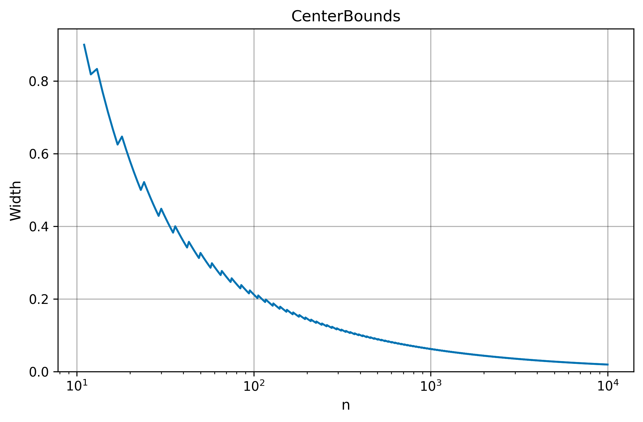
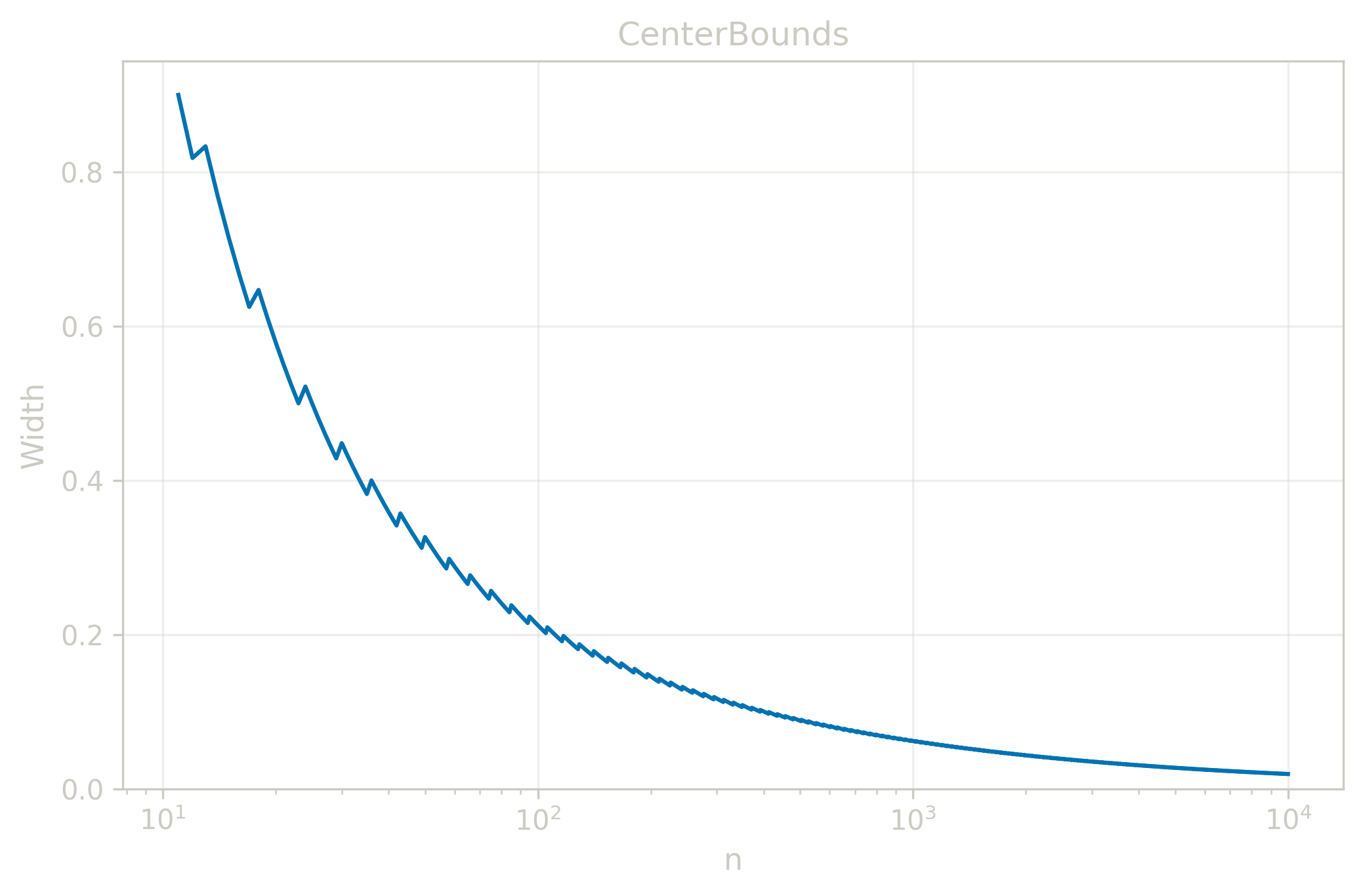
Width Convergence
The table below shows how narrows as grows, for ( evenly spaced points on ) and . Dashes indicate too small to achieve the target misrate.
| N | Width |
|---|---|
| 2 | — |
| 3 | — |
| 4 | — |
| 5 | — |
| 10 | — |
| 20 | 0.5789 |
| 30 | 0.4483 |
| 40 | 0.3590 |
| 50 | 0.3265 |
| 100 | 0.2121 |
| 200 | 0.1457 |
| 300 | 0.1171 |
| 400 | 0.1003 |
| 500 | 0.0882 |
| 1000 | 0.0621 |
| 10000 | 0.0192 |
Tests
where (pairwise averages, sorted) for , , , and .
The test suite contains 38 test cases (3 demo + 4 natural + 5 property + 7 edge + 4 symmetric + 2 additive + 2 uniform + 4 misrate + 6 unsorted + 1 error). Since returns bounds rather than a point estimate, tests validate that bounds contain and satisfy equivariance properties. Each test case output is a JSON object with lower and upper fields representing the interval bounds.
Demo examples — from manual introduction, validating basic bounds:
demo-1: , expected output:demo-2: , stricter fixture misrate, expected output:demo-3: , expected output:
These cases illustrate how tighter misrates produce wider bounds.
Natural sequences — 4 tests:
natural-5: , expected output:natural-7: , expected output:natural-10: , expected output:natural-20: , bounds containing
Property validation () — 5 tests:
property-identity: , expected output:property-centered: , expected output:property-location-shift: (= property-identity + 10), expected output: (location equivariance)property-scale-2x: , expected output:property-mixed-signs: , validates bounds crossing zero
Edge cases — boundary conditions and extreme scenarios (7 tests):
edge-two-elements: , minimum achievable misrate, expected output:edge-three-elements: (small sample)edge-loose-misrate: (permissive bounds)edge-strict-misrate: , stricter fixture misrateedge-duplicates-10: (all identical, bounds )edge-negative: (negative values)edge-wide-range: (extreme value range)
Symmetric distributions (varying fixture misrates) — 4 tests with symmetric data:
symmetric-5: , bounds centered aroundsymmetric-7: , bounds centered aroundsymmetric-10: symmetric aroundsymmetric-15: symmetric around
These tests validate that symmetric data produces symmetric bounds around the center.
Additive distribution (reference fixture misrates) — 2 tests with :
additive-10: , seed 0additive-20: , seed 0
Uniform distribution (reference fixture misrates) — 2 tests with :
uniform-10: , seed 1uniform-20: , seed 1
Misrate variation () — 4 tests with progressively stricter fixture misrates:
These tests validate monotonicity: smaller misrates produce wider bounds.
Unsorted tests — verify sorting independence (6 tests):
unsorted-reverse-5: , must equalnatural-5outputunsorted-reverse-7: , must equalnatural-7outputunsorted-shuffle-5: shuffled, must equal sorted counterpartunsorted-shuffle-7: shuffled, must equal sorted counterpartunsorted-negative-5: negative values unsortedunsorted-mixed-signs-5: mixed signs unsorted
These tests validate that produces identical results regardless of input order.
Error case — input validation:
error-empty-x: — empty array violates validity