ShiftBounds

where $\mathbf{z} = { x_i - y_j }$ (sorted), $k_{\text{left}} = \lfloor \operatorname{PairwiseMargin} / 2 \rfloor + 1$, $k_{\text{right}} = n m - \lfloor \operatorname{PairwiseMargin} / 2 \rfloor$

Robust bounds on $\operatorname{Shift}(\mathbf{x}, \mathbf{y})$ with specified coverage.

Input

• $\mathbf{x} = (x_1, x_2, \ldots, x_n)$ — first sample of measurements
• $\mathbf{y} = (y_1, y_2, \ldots, y_m)$ — second sample of measurements
• $\mathrm{misrate} \geq 2 / \binom{n+m}{n}$ — probability that true shift falls outside bounds in the long run

Output

• Value — interval $[L, U]$ bounding $\operatorname{Shift}(\mathbf{x}, \mathbf{y})$
• Unit — same unit as $\mathbf{x}$, $\mathbf{y}$

Notes

• Also known as — distribution-free confidence interval for Hodges-Lehmann
• Note — assumes weak continuity (ties from measurement resolution are tolerated but may yield conservative bounds)

Properties

• Shift invariance $\operatorname{ShiftBounds}(\mathbf{x} + k, \mathbf{y} + k, \mathrm{misrate}) = \operatorname{ShiftBounds}(\mathbf{x}, \mathbf{y}, \mathrm{misrate})$
• Scale equivariance $\operatorname{ShiftBounds}(k \cdot \mathbf{x}, k \cdot \mathbf{y}, \mathrm{misrate}) = k \cdot \operatorname{ShiftBounds}(\mathbf{x}, \mathbf{y}, \mathrm{misrate})$

Example

• ShiftBounds([1..30], [21..50], 1e-4) = [-30, -10] where Shift = -20
• Bounds fail to cover true shift with probability $\approx \mathrm{misrate}$

$\operatorname{ShiftBounds}$ provides not just the estimated shift but also the uncertainty of that estimate. The function returns an interval of plausible shift values given the data. Set $\mathrm{misrate}$ to control how often the bounds might fail to contain the true shift: use $10^{-3}$ for everyday analysis or $10^{-6}$ for critical decisions where errors are costly. These bounds require no assumptions about your data distribution, so they remain valid for any continuous measurements. If the bounds exclude zero, that suggests a reliable difference between the two groups.

See also: $\operatorname{Compare2}$ for comparing Shift against practical thresholds with automatic verdict generation.

Algorithm

The $\operatorname{ShiftBounds}$ estimator constructs distribution-free bounds on $\operatorname{Shift}(\mathbf{x}, \mathbf{y})$ by selecting specific order statistics from the pairwise differences.

Given samples $\mathbf{x} = (x_1, \ldots, x_n)$ and $\mathbf{y} = (y_1, \ldots, y_m)$, the algorithm proceeds as follows:

• Compute the margin Call $\operatorname{PairwiseMargin}(n, m, \mathrm{misrate})$ (see PairwiseMargin) to determine how many extreme pairwise differences to exclude from each tail.

• Determine quantile ranks From the margin $M$, compute $k_{\text{left}} = \lfloor M / 2 \rfloor + 1$ and $k_{\text{right}} = n m - \lfloor M / 2 \rfloor$. These are the ranks of the order statistics that form the bounds.

• Compute quantiles via Shift Use the Shift algorithm to compute the $k_{\text{left}}$-th and $k_{\text{right}}$-th order statistics of all $n m$ pairwise differences $x_i - y_j$. The Shift algorithms value-space binary search finds these quantiles in $O((n + m) \log L)$ time without materializing all differences.

• Return bounds Return $[z_{(k_{\text{left}})}, z_{(k_{\text{right}})}]$.

The $\operatorname{PairwiseMargin}$ function encodes the statistical theory: it determines which order statistics provide bounds with coverage $1 - \mathrm{misrate}$. The $\operatorname{Shift}$ algorithm provides the computational machinery: it extracts those specific order statistics efficiently from the implicit matrix of pairwise differences.

Notes

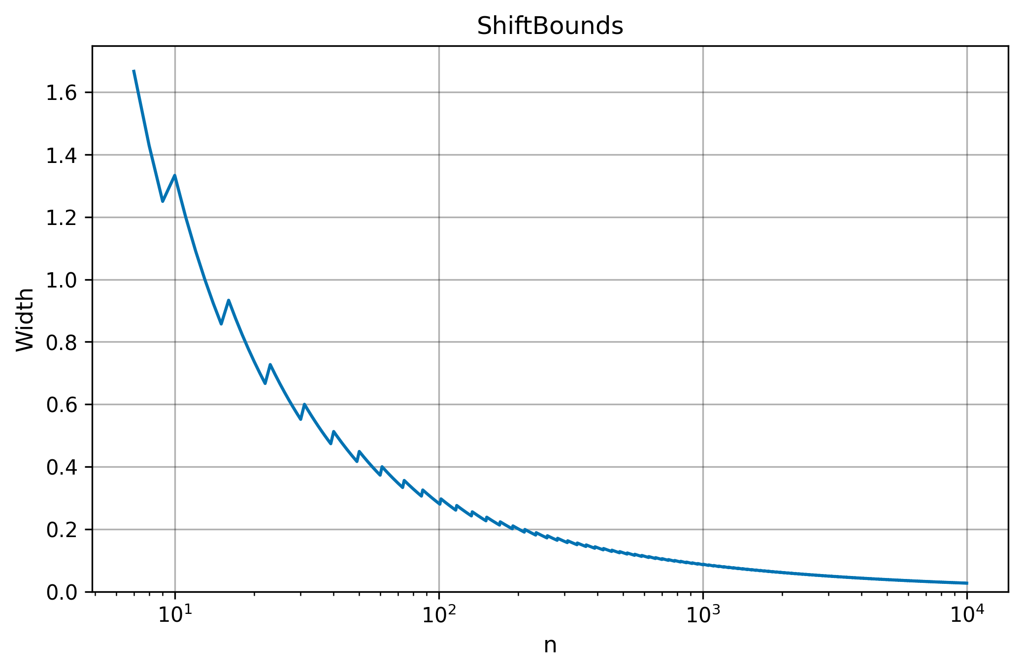
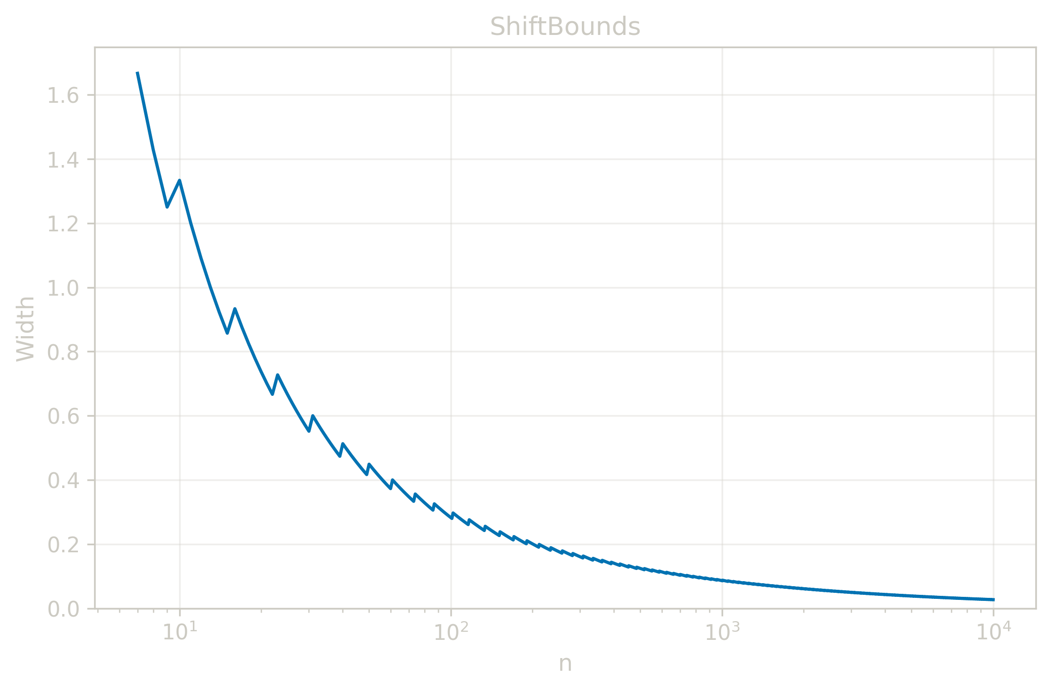
Width Convergence

The table below shows how $\text{Width} = U - L$ narrows as $N$ grows, for $\mathbf{x} = \mathbf{y} = (1, 1 + 1/(N-1), \ldots, 2)$ ($N$ evenly spaced points on $[1, 2]$) and $\mathrm{misrate} = 10^{-3}$. Dashes indicate $N$ too small to achieve the target misrate.

Tests

where

The $\operatorname{ShiftBounds}$ test suite contains 63 test cases (3 demo + 9 natural + 6 property + 10 edge + 9 additive + 4 uniform + 5 misrate + 15 unsorted + 2 error). Since $\operatorname{ShiftBounds}$ returns bounds rather than a point estimate, tests validate that the bounds contain $\operatorname{Shift}(\mathbf{x}, \mathbf{y})$ and satisfy equivariance properties. Each test case output is a JSON object with lower and upper fields representing the interval bounds. The domain constraint $\mathrm{misrate} \geq 2 / \binom{n+m}{n}$ is enforced; inputs violating this return a domain error.

Demo examples ($n = m = 5$) — from manual introduction, validating basic bounds:

• demo-1: $\mathbf{x} = (1, 2, 3, 4, 5)$, $\mathbf{y} = (3, 4, 5, 6, 7)$, expected output: $[-4, 0]$
• demo-2: $\mathbf{x} = (1, 2, 3, 4, 5)$, $\mathbf{y} = (3, 4, 5, 6, 7)$, stricter fixture misrate, expected output: $[-5, 1]$
• demo-3: $\mathbf{x} = (3, 4, 5, 6, 7)$, $\mathbf{y} = (3, 4, 5, 6, 7)$, expected output: bounds containing $0$ (identity case)

These cases illustrate how tighter misrates produce wider bounds and validate the identity property where identical samples yield bounds containing zero.

Natural sequences ($[n, m] in {5, 8, 10} \times {5, 8, 10}$, achievable fixture misrates) — 9 combinations:

• natural-5-5: $\mathbf{x} = (1, \ldots, 5)$, $\mathbf{y} = (1, \ldots, 5)$, expected bounds containing $0$
• natural-5-8: $\mathbf{x} = (1, \ldots, 5)$, $\mathbf{y} = (1, \ldots, 8)$
• natural-5-10: $\mathbf{x} = (1, \ldots, 5)$, $\mathbf{y} = (1, \ldots, 10)$
• natural-8-5: $\mathbf{x} = (1, \ldots, 8)$, $\mathbf{y} = (1, \ldots, 5)$
• natural-8-8: $\mathbf{x} = (1, \ldots, 8)$, $\mathbf{y} = (1, \ldots, 8)$, expected bounds containing $0$
• natural-8-10: $\mathbf{x} = (1, \ldots, 8)$, $\mathbf{y} = (1, \ldots, 10)$
• natural-10-5: $\mathbf{x} = (1, \ldots, 10)$, $\mathbf{y} = (1, \ldots, 5)$
• natural-10-8: $\mathbf{x} = (1, \ldots, 10)$, $\mathbf{y} = (1, \ldots, 8)$
• natural-10-10: $\mathbf{x} = (1, \ldots, 10)$, $\mathbf{y} = (1, \ldots, 10)$, expected bounds containing $0$

These sizes are chosen to satisfy $\mathrm{misrate} \geq 2 / \binom{n+m}{n}$ for all combinations.

Property validation ($n = m = 10$, $\mathrm{misrate} = 10^{-3}$) — 6 tests:

• property-identity: $\mathbf{x} = (0, 2, 4, \ldots, 18)$, $\mathbf{y} = (0, 2, 4, \ldots, 18)$, bounds must contain $0$
• property-location-shift: $\mathbf{x} = (7, 9, 11, \ldots, 25)$, $\mathbf{y} = (13, 15, 17, \ldots, 31)$
• Must produce same bounds as base case (location invariance)
• property-scale-2x: $\mathbf{x} = (2, 4, 6, \ldots, 20)$, $\mathbf{y} = (6, 8, 10, \ldots, 24)$
• Bounds must be 2× the base case bounds (scale equivariance)
• property-antisymmetry: $\mathbf{x} = (3, 4, \ldots, 12)$, $\mathbf{y} = (1, 2, \ldots, 10)$
• Bounds must be negated: if original is $[a, b]$, this yields $[-b, -a]$
• property-negative: $\mathbf{x} = (-10, -9, \ldots, -1)$, $\mathbf{y} = (-12, -11, \ldots, -3)$
• Validates sign handling with all negative values
• property-mixed-signs: $\mathbf{x} = (-4, -3, \ldots, 5)$, $\mathbf{y} = (-3, -2, \ldots, 6)$
• Validates bounds crossing zero with mixed-sign samples

Edge cases — boundary conditions and extreme scenarios (10 tests):

• edge-min-samples: $\mathbf{x} = (1, 2, 3, 4, 5)$, $\mathbf{y} = (6, 7, 8, 9, 10)$
• edge-permissive-misrate: $\mathbf{x} = (1, 2, 3, 4, 5)$, $\mathbf{y} = (3, 4, 5, 6, 7)$, very loose fixture misrate (very wide bounds)
• edge-strict-misrate: $n = m = 20$, $\mathrm{misrate} = 10^{-6}$ (very narrow bounds)
• edge-zero-shift: $n = m = 10$, all values $= 5$, $\mathrm{misrate} = 10^{-3}$ (bounds around 0)
• edge-asymmetric-3-100: $n = 3$, $m = 100$ (extreme size difference)
• edge-asymmetric-5-50: $n = 5$, $m = 50$, $\mathrm{misrate} = 10^{-3}$ (highly unbalanced)
• edge-duplicates: $\mathbf{x} = (3, 3, 3, 3, 3)$, $\mathbf{y} = (5, 5, 5, 5, 5)$ (all duplicates, bounds around 2)
• edge-wide-range: $n = m = 10$, values spanning $10^{-3}$ to $10^8$, $\mathrm{misrate} = 10^{-3}$ (extreme value range)
• edge-tiny-values: $n = m = 10$, values $\approx 10^{-8}$, $\mathrm{misrate} = 10^{-3}$ (numerical precision)
• edge-large-values: $n = m = 10$, values $\approx 10^8$, $\mathrm{misrate} = 10^{-3}$ (large magnitude)

These edge cases stress-test boundary conditions, numerical stability, and the margin calculation with extreme parameters.

Additive distribution ($[n, m] in {10, 30, 50} \times {10, 30, 50}$, $\mathrm{misrate} = 10^{-3}$) — 9 combinations with $\underline{\operatorname{Additive}}(10, 1)$:

• additive-10-10, additive-10-30, additive-10-50
• additive-30-10, additive-30-30, additive-30-50
• additive-50-10, additive-50-30, additive-50-50
• Random generation: $\mathbf{x}$ uses seed 0, $\mathbf{y}$ uses seed 1

These fuzzy tests validate that bounds properly encompass the shift estimate for realistic normally-distributed data at various sample sizes.

Uniform distribution ($[n, m] in {10, 100} \times {10, 100}$, $\mathrm{misrate} = 10^{-4}$) — 4 combinations with $\underline{\operatorname{Uniform}}(0, 1)$:

• uniform-10-10, uniform-10-100, uniform-100-10, uniform-100-100
• Random generation: $\mathbf{x}$ uses seed 2, $\mathbf{y}$ uses seed 3

The asymmetric size combinations are particularly important for testing margin calculation with unbalanced samples.

Misrate variation ($n = m = 20$, $\mathbf{x} = (0, 2, 4, \ldots, 38)$, $\mathbf{y} = (10, 12, 14, \ldots, 48)$) — 5 tests from a loose achievable fixture misrate down to $10^{-6}$:

These tests use identical samples with varying misrates to validate the monotonicity property: smaller misrates (higher confidence) produce wider bounds. The sequence demonstrates how bound width increases as misrate decreases, helping implementations verify correct margin calculation.

Unsorted tests — verify independent sorting of $\mathbf{x}$ and $\mathbf{y}$ (15 tests):

• unsorted-x-natural-5-5: $\mathbf{x} = (5, 3, 1, 4, 2)$, $\mathbf{y} = (1, 2, 3, 4, 5)$ (X reversed, Y sorted)
• unsorted-y-natural-5-5: $\mathbf{x} = (1, 2, 3, 4, 5)$, $\mathbf{y} = (5, 3, 1, 4, 2)$ (X sorted, Y reversed)
• unsorted-both-natural-5-5: $\mathbf{x} = (5, 3, 1, 4, 2)$, $\mathbf{y} = (5, 3, 1, 4, 2)$ (both reversed)
• unsorted-x-shuffle-5-5: $\mathbf{x} = (3, 1, 5, 4, 2)$, $\mathbf{y} = (1, 2, 3, 4, 5)$ (X shuffled)
• unsorted-y-shuffle-5-5: $\mathbf{x} = (1, 2, 3, 4, 5)$, $\mathbf{y} = (4, 2, 5, 1, 3)$ (Y shuffled)
• unsorted-both-shuffle-5-5: $\mathbf{x} = (3, 1, 5, 4, 2)$, $\mathbf{y} = (2, 4, 1, 5, 3)$ (both shuffled)
• unsorted-demo-unsorted-x: $\mathbf{x} = (5, 1, 4, 2, 3)$, $\mathbf{y} = (3, 4, 5, 6, 7)$ (demo-1 X unsorted)
• unsorted-demo-unsorted-y: $\mathbf{x} = (1, 2, 3, 4, 5)$, $\mathbf{y} = (7, 3, 6, 4, 5)$ (demo-1 Y unsorted)
• unsorted-demo-both-unsorted: $\mathbf{x} = (4, 1, 5, 2, 3)$, $\mathbf{y} = (6, 3, 7, 4, 5)$ (demo-1 both unsorted)
• unsorted-identity-unsorted: $\mathbf{x} = (4, 1, 5, 2, 3)$, $\mathbf{y} = (5, 1, 4, 3, 2)$ (identity property, both unsorted)
• unsorted-negative-unsorted: $\mathbf{x} = (-1, -5, -3, -2, -4)$, $\mathbf{y} = (-2, -4, -3, -5, -1)$ (negative values unsorted)
• unsorted-asymmetric-5-10: $\mathbf{x} = (2, 5, 1, 3, 4)$, $\mathbf{y} = (10, 5, 2, 8, 4, 1, 9, 3, 7, 6)$ (asymmetric sizes, both unsorted)
• unsorted-duplicates: $\mathbf{x} = (3, 3, 3, 3, 3)$, $\mathbf{y} = (5, 5, 5, 5, 5)$ (all duplicates, any order)
• unsorted-mixed-duplicates-x: $\mathbf{x} = (2, 1, 3, 2, 1)$, $\mathbf{y} = (1, 1, 2, 2, 3)$ (X has unsorted duplicates)
• unsorted-mixed-duplicates-y: $\mathbf{x} = (1, 1, 2, 2, 3)$, $\mathbf{y} = (3, 2, 1, 3, 2)$ (Y has unsorted duplicates)

These unsorted tests are critical because $\operatorname{ShiftBounds}$ computes bounds from pairwise differences, requiring both samples to be sorted independently. The variety ensures implementations dont incorrectly assume pre-sorted input or sort samples together. Each test must produce identical output to its sorted counterpart, validating that the implementation correctly handles the sorting step.

Error cases — input validation (2 tests):

• error-empty-x: $\mathbf{x} = ()$, $\mathbf{y} = (1, 2, 3, 4, 5)$ — empty X array violates validity
• error-empty-y: $\mathbf{x} = (1, 2, 3, 4, 5)$, $\mathbf{y} = ()$ — empty Y array violates validity

No performance test — $\operatorname{ShiftBounds}$ uses the $\text{FastShift}$ algorithm internally, which is already validated by the $\operatorname{Shift}$ performance test. Since bounds computation involves only two quantile calculations from the pairwise differences (at positions determined by $\operatorname{PairwiseMargin}$), the performance characteristics are equivalent to computing two $\operatorname{Shift}$ estimates, which completes efficiently for large samples.