RatioBounds

Robust bounds on $\operatorname{Ratio}(\mathbf{x}, \mathbf{y})$ with specified coverage — the multiplicative dual of $\operatorname{ShiftBounds}$.

Input

• $\mathbf{x} = (x_1, x_2, \ldots, x_n)$ — first sample of measurements, where $x_i > 0$, requires positivity(x)
• $\mathbf{y} = (y_1, y_2, \ldots, y_m)$ — second sample of measurements, where $y_j > 0$, requires positivity(y)
• $\mathrm{misrate} \geq 2 / \binom{n+m}{n}$ — probability that true ratio falls outside bounds in the long run

Output

• Value — interval $[L, U]$ bounding $\operatorname{Ratio}(\mathbf{x}, \mathbf{y})$
• Unit — dimensionless

Notes

• Also known as — distribution-free confidence interval for Hodges-Lehmann ratio
• Note — assumes weak continuity (ties from measurement resolution are tolerated but may yield conservative bounds)

Properties

• Scale invariance $\operatorname{RatioBounds}(k \cdot \mathbf{x}, k \cdot \mathbf{y}, \mathrm{misrate}) = \operatorname{RatioBounds}(\mathbf{x}, \mathbf{y}, \mathrm{misrate})$
• Scale equivariance $\operatorname{RatioBounds}(k_x \cdot \mathbf{x}, k_y \cdot \mathbf{y}, \mathrm{misrate}) = (k_x / k_y) \cdot \operatorname{RatioBounds}(\mathbf{x}, \mathbf{y}, \mathrm{misrate})$
• Multiplicative antisymmetry $\operatorname{RatioBounds}(\mathbf{x}, \mathbf{y}, \mathrm{misrate}) = 1 / \operatorname{RatioBounds}(\mathbf{y}, \mathbf{x}, \mathrm{misrate})$ (bounds reversed)

Example

• RatioBounds([1..30], [10..40], 1e-4) where Ratio ≈ 0.5 yields bounds containing $0.5$
• Bounds fail to cover true ratio with probability $\approx \mathrm{misrate}$

Relationship to ShiftBounds

$\operatorname{RatioBounds}$ is computed via log-transformation:

This means if $\operatorname{ShiftBounds}$ returns $[a, b]$ for the log-transformed samples, $\operatorname{RatioBounds}$ returns $[e^a, e^b]$.

$\operatorname{RatioBounds}$ provides not just the estimated ratio but also the uncertainty of that estimate. The function returns an interval of plausible ratio values given the data. Set $\mathrm{misrate}$ to control how often the bounds might fail to contain the true ratio: use $10^{-3}$ for everyday analysis or $10^{-6}$ for critical decisions where errors are costly. These bounds require no assumptions about your data distribution, so they remain valid for any continuous positive measurements. If the bounds exclude $1$, that suggests a reliable multiplicative difference between the two groups.

See also: $\operatorname{Compare2}$ for comparing Ratio against practical thresholds with automatic verdict generation.

Algorithm

The $\operatorname{RatioBounds}$ estimator uses the same log-exp transformation as Ratio, delegating to ShiftBounds in log-space:

The algorithm operates in three steps:

• Log-transform Apply $\log$ to each element of both samples. Positivity is required so that the logarithm is defined.

• Delegate to ShiftBounds Compute $[a, b] = \operatorname{ShiftBounds}(\log \mathbf{x}, \log \mathbf{y}, \mathrm{misrate})$. This provides distribution-free bounds on the shift in log-space.

• Exp-transform Return $[e^a, e^b]$, converting the additive bounds back to multiplicative bounds.

Because $\log$ and $\exp$ are monotone, the coverage guarantee of $\operatorname{ShiftBounds}$ transfers directly: the probability that the true ratio falls outside $[e^a, e^b]$ equals the probability that the true log-shift falls outside $[a, b]$, which is at most $\mathrm{misrate}$.

Notes

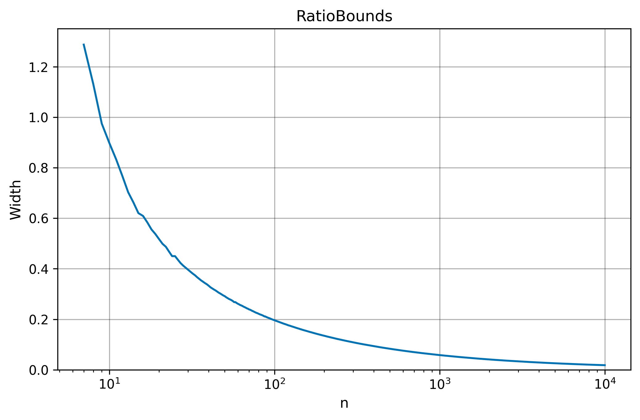
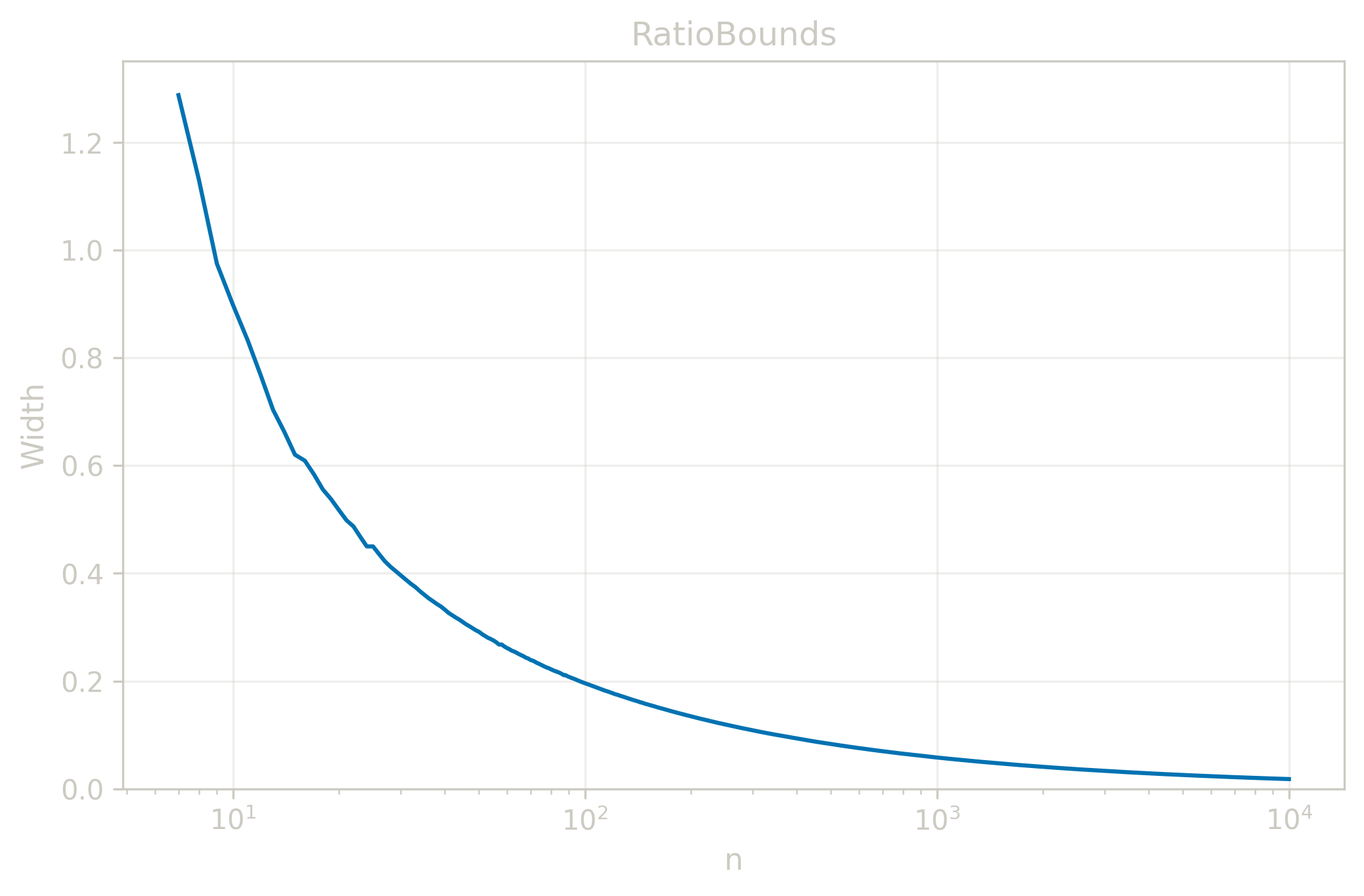
Width Convergence

The table below shows how $\text{Width} = U - L$ narrows as $N$ grows, for $\mathbf{x} = \mathbf{y} = (1, 1 + 1/(N-1), \ldots, 2)$ ($N$ evenly spaced points on $[1, 2]$) and $\mathrm{misrate} = 10^{-3}$. Dashes indicate $N$ too small to achieve the target misrate.

Tests

The $\operatorname{RatioBounds}$ test suite contains 63 test cases (3 demo + 9 natural + 6 property + 10 edge + 9 multiplic + 4 uniform + 5 misrate + 15 unsorted + 2 error). Since $\operatorname{RatioBounds}$ returns bounds rather than a point estimate, tests validate that the bounds contain $\operatorname{Ratio}(\mathbf{x}, \mathbf{y})$ and satisfy equivariance properties. Each test case output is a JSON object with lower and upper fields representing the interval bounds. All samples must contain strictly positive values. The domain constraint $\mathrm{misrate} \geq 2 / \binom{n+m}{n}$ is enforced; inputs violating this return a domain error.

Demo examples ($n = m = 5$, positive samples) — 3 tests:

• demo-1: $\mathbf{x} = (1, 2, 3, 4, 5)$, $\mathbf{y} = (2, 3, 4, 5, 6)$
• demo-2: $\mathbf{x} = (1, 2, 3, 4, 5)$, $\mathbf{y} = (2, 3, 4, 5, 6)$, stricter fixture misrate, expected: wider bounds than demo-1
• demo-3: $\mathbf{x} = (2, 3, 4, 5, 6)$, $\mathbf{y} = (2, 3, 4, 5, 6)$, expected: bounds containing $1$ (identity case)

These cases illustrate how tighter misrates produce wider bounds and validate the identity property where identical samples yield bounds containing one.

Natural sequences ($[n, m] in {5, 8, 10} \times {5, 8, 10}$, achievable fixture misrates) — 9 combinations:

• natural-5-5: $\mathbf{x} = (1, \ldots, 5)$, $\mathbf{y} = (1, \ldots, 5)$, expected bounds containing $1$
• natural-5-8: $\mathbf{x} = (1, \ldots, 5)$, $\mathbf{y} = (1, \ldots, 8)$
• natural-5-10: $\mathbf{x} = (1, \ldots, 5)$, $\mathbf{y} = (1, \ldots, 10)$
• natural-8-5: $\mathbf{x} = (1, \ldots, 8)$, $\mathbf{y} = (1, \ldots, 5)$
• natural-8-8: $\mathbf{x} = (1, \ldots, 8)$, $\mathbf{y} = (1, \ldots, 8)$, expected bounds containing $1$
• natural-8-10: $\mathbf{x} = (1, \ldots, 8)$, $\mathbf{y} = (1, \ldots, 10)$
• natural-10-5: $\mathbf{x} = (1, \ldots, 10)$, $\mathbf{y} = (1, \ldots, 5)$
• natural-10-8: $\mathbf{x} = (1, \ldots, 10)$, $\mathbf{y} = (1, \ldots, 8)$
• natural-10-10: $\mathbf{x} = (1, \ldots, 10)$, $\mathbf{y} = (1, \ldots, 10)$, expected bounds containing $1$

These sizes are chosen to satisfy $\mathrm{misrate} \geq 2 / \binom{n+m}{n}$ for all combinations.

Property validation ($n = m = 10$, $\mathrm{misrate} = 10^{-3}$) — 6 tests:

• property-identity: $\mathbf{x} = (1, 2, \ldots, 10)$, $\mathbf{y} = (1, 2, \ldots, 10)$, bounds must contain $1$
• property-scale-2x: $\mathbf{x} = (2, 4, \ldots, 20)$, $\mathbf{y} = (1, 2, \ldots, 10)$, bounds must contain $2$
• property-reciprocal: $\mathbf{x} = (1, 2, \ldots, 10)$, $\mathbf{y} = (2, 4, \ldots, 20)$, bounds must contain $0.5$ (reciprocal of scale-2x)
• property-common-scale: $\mathbf{x} = (10, 20, \ldots, 100)$, $\mathbf{y} = (20, 40, \ldots, 200)$
• Same ratio as property-reciprocal (common scale invariance)
• property-small-values: $\mathbf{x} = (0.1, 0.2, \ldots, 1.0)$, $\mathbf{y} = (0.2, 0.4, \ldots, 2.0)$
• Same ratio as property-reciprocal (small value handling)
• property-mixed-scales: $\mathbf{x} = (0.01, 0.1, 1, 10, 100, 1000, 0.5, 5, 50, 500)$, $\mathbf{y} = (0.1, 1, 10, 100, 1000, 10000, 5, 50, 500, 5000)$
• Wide range validation

Edge cases — boundary conditions and extreme scenarios (10 tests):

• edge-min-samples: $\mathbf{x} = (2, 3, 4, 5, 6)$, $\mathbf{y} = (3, 4, 5, 6, 7)$
• edge-permissive-misrate: $\mathbf{x} = (1, 2, 3, 4, 5)$, $\mathbf{y} = (2, 3, 4, 5, 6)$, very loose fixture misrate (very wide bounds)
• edge-strict-misrate: $n = m = 20$, $\mathrm{misrate} = 10^{-6}$ (very narrow bounds)
• edge-unity-ratio: $n = m = 10$, all values $= 5$, $\mathrm{misrate} = 10^{-3}$ (bounds around 1)
• edge-asymmetric-3-100: $n = 3$, $m = 100$ (extreme size difference)
• edge-asymmetric-5-50: $n = 5$, $m = 50$, $\mathrm{misrate} = 10^{-3}$ (highly unbalanced)
• edge-duplicates: $\mathbf{x} = (3, 3, 3, 3, 3)$, $\mathbf{y} = (5, 5, 5, 5, 5)$ (all duplicates, bounds around 0.6)
• edge-wide-range: $n = m = 10$, values spanning $10^{-3}$ to $10^8$, $\mathrm{misrate} = 10^{-3}$ (extreme value range)
• edge-tiny-values: $n = m = 10$, values $\approx 10^{-6}$, $\mathrm{misrate} = 10^{-3}$ (numerical precision)
• edge-large-values: $n = m = 10$, values $\approx 10^8$, $\mathrm{misrate} = 10^{-3}$ (large magnitude)

These edge cases stress-test boundary conditions, numerical stability, and the margin calculation with extreme parameters.

Multiplic distribution ($[n, m] in {10, 30, 50} \times {10, 30, 50}$, $\mathrm{misrate} = 10^{-3}$) — 9 combinations with $\underline{\operatorname{Multiplic}}(1, 0.5)$:

• multiplic-10-10, multiplic-10-30, multiplic-10-50
• multiplic-30-10, multiplic-30-30, multiplic-30-50
• multiplic-50-10, multiplic-50-30, multiplic-50-50
• Random generation: $\mathbf{x}$ uses seed 0, $\mathbf{y}$ uses seed 1

These fuzzy tests validate that bounds properly encompass the ratio estimate for realistic log-normally-distributed data at various sample sizes.

Uniform distribution ($[n, m] in {10, 100} \times {10, 100}$, $\mathrm{misrate} = 10^{-4}$) — 4 combinations with $\underline{\operatorname{Uniform}}(1, 10)$:

• uniform-10-10, uniform-10-100, uniform-100-10, uniform-100-100
• Random generation: $\mathbf{x}$ uses seed 2, $\mathbf{y}$ uses seed 3
• Note: positive range $[1, 10)$ used for ratio compatibility

The asymmetric size combinations are particularly important for testing margin calculation with unbalanced samples.

Misrate variation ($n = m = 20$, $\mathbf{x} = (1, 2, \ldots, 20)$, $\mathbf{y} = (2, 4, \ldots, 40)$) — 5 tests from a loose achievable fixture misrate down to $10^{-6}$:

These tests use identical samples with varying misrates to validate the monotonicity property: smaller misrates produce wider bounds. The sequence demonstrates how bound width increases as misrate decreases, helping implementations verify correct margin calculation.

Unsorted tests — verify independent sorting of $\mathbf{x}$ and $\mathbf{y}$ (15 tests):

• unsorted-x-natural-5-5: $\mathbf{x} = (5, 3, 1, 4, 2)$, $\mathbf{y} = (1, 2, 3, 4, 5)$ (X reversed, Y sorted)
• unsorted-y-natural-5-5: $\mathbf{x} = (1, 2, 3, 4, 5)$, $\mathbf{y} = (5, 3, 1, 4, 2)$ (X sorted, Y reversed)
• unsorted-both-natural-5-5: $\mathbf{x} = (5, 3, 1, 4, 2)$, $\mathbf{y} = (5, 3, 1, 4, 2)$ (both reversed)
• unsorted-x-shuffle-5-5: $\mathbf{x} = (3, 1, 5, 4, 2)$, $\mathbf{y} = (1, 2, 3, 4, 5)$ (X shuffled)
• unsorted-y-shuffle-5-5: $\mathbf{x} = (1, 2, 3, 4, 5)$, $\mathbf{y} = (4, 2, 5, 1, 3)$ (Y shuffled)
• unsorted-both-shuffle-5-5: $\mathbf{x} = (3, 1, 5, 4, 2)$, $\mathbf{y} = (2, 4, 1, 5, 3)$ (both shuffled)
• unsorted-demo-unsorted-x: $\mathbf{x} = (5, 1, 4, 2, 3)$, $\mathbf{y} = (2, 3, 4, 5, 6)$ (demo-1 X unsorted)
• unsorted-demo-unsorted-y: $\mathbf{x} = (1, 2, 3, 4, 5)$, $\mathbf{y} = (6, 2, 5, 3, 4)$ (demo-1 Y unsorted)
• unsorted-demo-both-unsorted: $\mathbf{x} = (4, 1, 5, 2, 3)$, $\mathbf{y} = (5, 2, 6, 3, 4)$ (demo-1 both unsorted)
• unsorted-identity-unsorted: $\mathbf{x} = (4, 1, 5, 2, 3)$, $\mathbf{y} = (5, 1, 4, 3, 2)$ (identity property, both unsorted)
• unsorted-scale-unsorted: $\mathbf{x} = (10, 30, 20)$, $\mathbf{y} = (15, 5, 10)$ (scale relationship, both unsorted)
• unsorted-asymmetric-5-10: $\mathbf{x} = (2, 5, 1, 3, 4)$, $\mathbf{y} = (10, 5, 2, 8, 4, 1, 9, 3, 7, 6)$ (asymmetric sizes, both unsorted)
• unsorted-duplicates: $\mathbf{x} = (3, 3, 3, 3, 3)$, $\mathbf{y} = (5, 5, 5, 5, 5)$ (all duplicates, any order)
• unsorted-mixed-duplicates-x: $\mathbf{x} = (2, 1, 3, 2, 1)$, $\mathbf{y} = (1, 1, 2, 2, 3)$ (X has unsorted duplicates)
• unsorted-mixed-duplicates-y: $\mathbf{x} = (1, 1, 2, 2, 3)$, $\mathbf{y} = (3, 2, 1, 3, 2)$ (Y has unsorted duplicates)

These unsorted tests are critical because $\operatorname{RatioBounds}$ computes bounds from pairwise ratios, requiring both samples to be sorted independently. The variety ensures implementations dont incorrectly assume pre-sorted input or sort samples together. Each test must produce identical output to its sorted counterpart, validating that the implementation correctly handles the sorting step.

Error cases — input validation (2 tests):

• error-empty-x: $\mathbf{x} = ()$, $\mathbf{y} = (1, 2, 3, 4, 5)$ — empty X array violates validity
• error-empty-y: $\mathbf{x} = (1, 2, 3, 4, 5)$, $\mathbf{y} = ()$ — empty Y array violates validity

No performance test — $\operatorname{RatioBounds}$ uses the $\text{FastRatio}$ algorithm internally, which delegates to $\text{FastShift}$ in log-space. Since bounds computation involves only two quantile calculations from the pairwise differences (at positions determined by $\operatorname{PairwiseMargin}$), the performance characteristics are equivalent to computing two $\operatorname{Ratio}$ estimates, which completes efficiently for large samples.