Spread

Robust measure of dispersion (variability, scatter).

• Also known as — Shamos scale estimator
• Asymptotic — median of the absolute difference between two random measurements from $X$
• Complexity — $O(n \log n)$
• Domain — any real numbers
• Assumptions — sparity(x)
• Unit — same as measurements

Properties

• Shift invariance $\operatorname{Spread}(\mathbf{x} + k) = \operatorname{Spread}(\mathbf{x})$
• Scale equivariance $\operatorname{Spread}(k \cdot \mathbf{x}) = \lvert k \rvert \cdot \operatorname{Spread}(\mathbf{x})$
• Non-negativity $\operatorname{Spread}(\mathbf{x}) \geq 0$

Example

• Spread([0, 2, 4, 6, 8]) = 4
• Spread(x + 10) = 4 Spread(2x) = 8

$\operatorname{Spread}$ measures how much measurements vary from each other. It serves the same purpose as standard deviation but does not explode with outliers or heavy-tailed data. The result comes in the same units as the measurements, so if $\operatorname{Spread}$ is 5 milliseconds, that indicates how much values typically differ. Like $\operatorname{Center}$, it tolerates up to 29% corrupted data. When comparing variability across datasets, $\operatorname{Spread}$ gives a reliable answer even when standard deviation would be misleading or infinite. When all values are positive, $\operatorname{Spread}$ can be conveniently expressed in relative units by dividing by $\lvert \operatorname{Center} \rvert$: the ratio $\frac{\operatorname{Spread}(\mathbf{x})}{\lvert \operatorname{Center}(\mathbf{x}) \rvert}$ is a robust alternative to the coefficient of variation that is scale-invariant.

Algorithm

The $\operatorname{Spread}$ estimator computes the median of all pairwise absolute differences. Given a sample $x = (x_1, x_2, \ldots, x_n)$, this estimator is defined as:

Like $\operatorname{Center}$, computing $\operatorname{Spread}$ naively requires generating all $\frac{n(n-1)}{2}$ pairwise differences, sorting them, and finding the median — a quadratic approach that becomes computationally prohibitive for large datasets.

The same structural principles that accelerate $\operatorname{Center}$ computation also apply to pairwise differences, yielding an exact $O(n \log n)$ algorithm. After sorting the input to obtain $y_1 \leq y_2 \leq \ldots \leq y_n$, all pairwise absolute differences $\lvert x_i - x_j \rvert$ with $i < j$ become positive differences $y_j - y_i$. This allows considering the implicit upper triangular matrix $D$ where $D_{i,j} = y_j - y_i$ for $i < j$. This matrix has a crucial structural property: for a fixed row $i$, differences increase monotonically, while for a fixed column $j$, differences decrease as $i$ increases. This sorted structure enables linear-time counting of elements below any threshold.

The algorithm applies Monahans selection strategy (Monahan 1984), adapted for differences rather than sums. For each row $i$, it tracks active column indices representing differences still under consideration, initially spanning columns $i+1$ through $n$. It chooses candidate differences from the active set using weighted random row selection, maintaining expected logarithmic convergence while avoiding expensive pivot computations. For any pivot value $p$, the number of differences falling below $p$ is counted using a single sweep; the monotonic structure ensures this counting requires only $O(n)$ operations. While counting, the largest difference below $p$ and the smallest difference at or above $p$ are maintained — these boundary values become the exact answer when the target rank is reached.

The algorithm naturally handles both odd and even cases. For an odd number of differences, it returns the single middle element when the count exactly hits the median rank. For an even number of differences, it returns the average of the two middle elements; boundary tracking during counting provides both values simultaneously. Unlike approximation methods, this algorithm returns the precise median of all pairwise differences; randomness affects only performance, not correctness.

The algorithm includes the same stall-handling mechanisms as the center algorithm. It tracks whether the count below the pivot changes between iterations; when progress stalls due to tied values, it computes the range of remaining active differences and pivots to their midrange. This midrange strategy ensures convergence even with highly discrete data or datasets with many identical values.

Several optimizations make the implementation practical for production use. A global column pointer that never moves backward during counting exploits the matrix structure to avoid redundant comparisons. Exact boundary values are captured during each counting pass, eliminating the need for additional searches when the target rank is reached. Using only $O(n)$ additional space for row bounds and counters, the algorithm achieves $O(n \log n)$ time complexity with minimal memory overhead, making robust scale estimation practical for large datasets.

namespace Pragmastat.Algorithms;

internal static class FastSpread
{
  /// <summary>
  /// Shamos "Spread".  Expected O(n log n) time, O(n) extra space. Exact.
  /// </summary>
  public static double Estimate(IReadOnlyList<double> values, Random? random = null, bool isSorted = false)
  {
    int n = values.Count;
    if (n <= 1) return 0;
    if (n == 2) return Abs(values[1] - values[0]);
    random ??= new Random();

    // Prepare a sorted working copy.
    double[] a = isSorted ? CopySorted(values) : EnsureSorted(values);

    // Total number of pairwise differences with i < j
    long N = (long)n * (n - 1) / 2;
    long kLow = (N + 1) / 2; // 1-based rank of lower middle
    long kHigh = (N + 2) / 2; // 1-based rank of upper middle

    // Per-row active bounds over columns j (0-based indices).
    // Row i allows j in [i+1, n-1] initially.
    int[] L = new int[n];
    int[] R = new int[n];
    long[] rowCounts = new long[n]; // # of elements in row i that are < pivot (for current partition)

    for (int i = 0; i < n; i++)
    {
      L[i] = Min(i + 1, n); // n means empty
      R[i] = n - 1; // inclusive
      if (L[i] > R[i])
      {
        L[i] = 1;
        R[i] = 0;
      } // mark empty
    }

    // A reasonable initial pivot: a central gap
    double pivot = a[n / 2] - a[(n - 1) / 2];

    long prevCountBelow = -1;

    while (true)
    {
      // === PARTITION: count how many differences are < pivot; also track boundary neighbors ===
      long countBelow = 0;
      double largestBelow = double.NegativeInfinity; // max difference < pivot
      double smallestAtOrAbove = double.PositiveInfinity; // min difference >= pivot

      int j = 1; // global two-pointer (non-decreasing across rows)
      for (int i = 0; i < n - 1; i++)
      {
        if (j < i + 1) j = i + 1;
        while (j < n && a[j] - a[i] < pivot) j++;

        long cntRow = j - (i + 1);
        if (cntRow < 0) cntRow = 0;
        rowCounts[i] = cntRow;
        countBelow += cntRow;

        // boundary elements for this row
        if (cntRow > 0)
        {
          // last < pivot in this row is (j-1)
          double candBelow = a[j - 1] - a[i];
          if (candBelow > largestBelow) largestBelow = candBelow;
        }

        if (j < n)
        {
          double candAtOrAbove = a[j] - a[i];
          if (candAtOrAbove < smallestAtOrAbove) smallestAtOrAbove = candAtOrAbove;
        }
      }

      // === TARGET CHECK ===
      // If we've split exactly at the middle, we can return using the boundaries we just found.
      bool atTarget =
        (countBelow == kLow) || // lower middle is the largest < pivot
        (countBelow == (kHigh - 1)); // upper middle is the smallest >= pivot

      if (atTarget)
      {
        if (kLow < kHigh)
        {
          // Even N: average the two central order stats.
          return 0.5 * (largestBelow + smallestAtOrAbove);
        }
        else
        {
          // Odd N: pick the single middle depending on which side we hit.
          bool needLargest = (countBelow == kLow);
          return needLargest ? largestBelow : smallestAtOrAbove;
        }
      }

      // === STALL HANDLING (ties / no progress) ===
      if (countBelow == prevCountBelow)
      {
        // Compute min/max remaining difference in the ACTIVE set and pivot to their midrange.
        double minActive = double.PositiveInfinity;
        double maxActive = double.NegativeInfinity;
        long active = 0;

        for (int i = 0; i < n - 1; i++)
        {
          int Li = L[i], Ri = R[i];
          if (Li > Ri) continue;

          double rowMin = a[Li] - a[i];
          double rowMax = a[Ri] - a[i];
          if (rowMin < minActive) minActive = rowMin;
          if (rowMax > maxActive) maxActive = rowMax;
          active += (Ri - Li + 1);
        }

        if (active <= 0)
        {
          // No active candidates left: the only consistent answer is the boundary implied by counts.
          // Fall back to neighbors from this partition.
          if (kLow < kHigh) return 0.5 * (largestBelow + smallestAtOrAbove);
          return (countBelow >= kLow) ? largestBelow : smallestAtOrAbove;
        }

        if (maxActive <= minActive) return minActive; // all remaining equal

        double mid = 0.5 * (minActive + maxActive);
        pivot = (mid > minActive && mid <= maxActive) ? mid : maxActive;
        prevCountBelow = countBelow;
        continue;
      }

      // === SHRINK ACTIVE WINDOW ===
      // --- SHRINK ACTIVE WINDOW (fixed) ---
      if (countBelow < kLow)
      {
        // Need larger differences: discard all strictly below pivot.
        for (int i = 0; i < n - 1; i++)
        {
          // First j with a[j] - a[i] >= pivot is j = i + 1 + cntRow (may be n => empty row)
          int newL = i + 1 + (int)rowCounts[i];
          if (newL > L[i]) L[i] = newL; // do NOT clamp; allow L[i] == n to mean empty
          if (L[i] > R[i])
          {
            L[i] = 1;
            R[i] = 0;
          } // mark empty
        }
      }
      else
      {
        // Too many below: keep only those strictly below pivot.
        for (int i = 0; i < n - 1; i++)
        {
          // Last j with a[j] - a[i] < pivot is j = i + cntRow  (not cntRow-1!)
          int newR = i + (int)rowCounts[i];
          if (newR < R[i]) R[i] = newR; // shrink downward to the true last-below
          if (R[i] < i + 1)
          {
            L[i] = 1;
            R[i] = 0;
          } // empty row if none remain
        }
      }

      prevCountBelow = countBelow;

      // === CHOOSE NEXT PIVOT FROM ACTIVE SET (weighted random row, then row median) ===
      long activeSize = 0;
      for (int i = 0; i < n - 1; i++)
      {
        if (L[i] <= R[i]) activeSize += (R[i] - L[i] + 1);
      }

      if (activeSize <= 2)
      {
        // Few candidates left: return midrange of remaining exactly.
        double minRem = double.PositiveInfinity, maxRem = double.NegativeInfinity;
        for (int i = 0; i < n - 1; i++)
        {
          if (L[i] > R[i]) continue;
          double lo = a[L[i]] - a[i];
          double hi = a[R[i]] - a[i];
          if (lo < minRem) minRem = lo;
          if (hi > maxRem) maxRem = hi;
        }

        if (activeSize <= 0) // safety net; fall back to boundary from last partition
        {
          if (kLow < kHigh) return 0.5 * (largestBelow + smallestAtOrAbove);
          return (countBelow >= kLow) ? largestBelow : smallestAtOrAbove;
        }

        if (kLow < kHigh) return 0.5 * (minRem + maxRem);
        return (Abs((kLow - 1) - countBelow) <= Abs(countBelow - kLow)) ? minRem : maxRem;
      }
      else
      {
        long t = NextIndex(random, activeSize); // 0..activeSize-1
        long acc = 0;
        int row = 0;
        for (; row < n - 1; row++)
        {
          if (L[row] > R[row]) continue;
          long size = R[row] - L[row] + 1;
          if (t < acc + size) break;
          acc += size;
        }

        // Median column of the selected row
        int col = (L[row] + R[row]) >> 1;
        pivot = a[col] - a[row];
      }
    }
  }
  // --- Helpers ---

  private static double[] CopySorted(IReadOnlyList<double> values)
  {
    var a = new double[values.Count];
    for (int i = 0; i < a.Length; i++)
    {
      double v = values[i];
      if (double.IsNaN(v)) throw new ArgumentException("NaN not allowed.", nameof(values));
      a[i] = v;
    }

    Array.Sort(a);
    return a;
  }

  private static double[] EnsureSorted(IReadOnlyList<double> values)
  {
    // Trust caller; still copy to array for fast indexed access.
    var a = new double[values.Count];
    for (int i = 0; i < a.Length; i++)
    {
      double v = values[i];
      if (double.IsNaN(v)) throw new ArgumentException("NaN not allowed.", nameof(values));
      a[i] = v;
    }

    return a;
  }

  private static long NextIndex(Random rng, long limitExclusive)
  {
    // Uniform 0..limitExclusive-1 even for large ranges.
    // Use rejection sampling for correctness.
    ulong uLimit = (ulong)limitExclusive;
    if (uLimit <= int.MaxValue)
    {
      return rng.Next((int)uLimit);
    }

    while (true)
    {
      ulong u = ((ulong)(uint)rng.Next() << 32) | (uint)rng.Next();
      ulong r = u % uLimit;
      if (u - r <= ulong.MaxValue - (ulong.MaxValue % uLimit)) return (long)r;
    }
  }
}

Notes

This section compares the toolkits robust dispersion estimator against traditional methods to demonstrate its advantages across diverse conditions.

Dispersion Estimators

Standard Deviation:

Median Absolute Deviation (around the median):

Spread (Shamos scale estimator):

Breakdown

Heavy-tailed distributions naturally produce extreme outliers that completely distort traditional estimators. A single extreme measurement from the $\underline{\operatorname{Power}}$ distribution can make the standard deviation arbitrarily large. Real-world data can also contain corrupted measurements from instrument failures, recording errors, or transmission problems. Both natural extremes and data corruption create the same challenge: extracting reliable information when some measurements are too influential.

The breakdown point (Huber 2009) is the fraction of a sample that can be replaced by arbitrarily large values without making an estimator arbitrarily large. The theoretical maximum is $50\%$; no estimator can guarantee reliable results when more than half the measurements are extreme or corrupted.

The $\operatorname{Spread}$ estimator achieves a $29\%$ breakdown point, providing substantial protection against realistic contamination levels while maintaining good precision.

Asymptotic breakdown points for dispersion estimators:

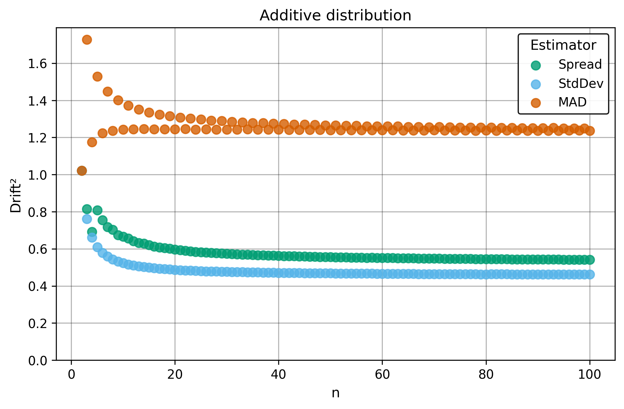
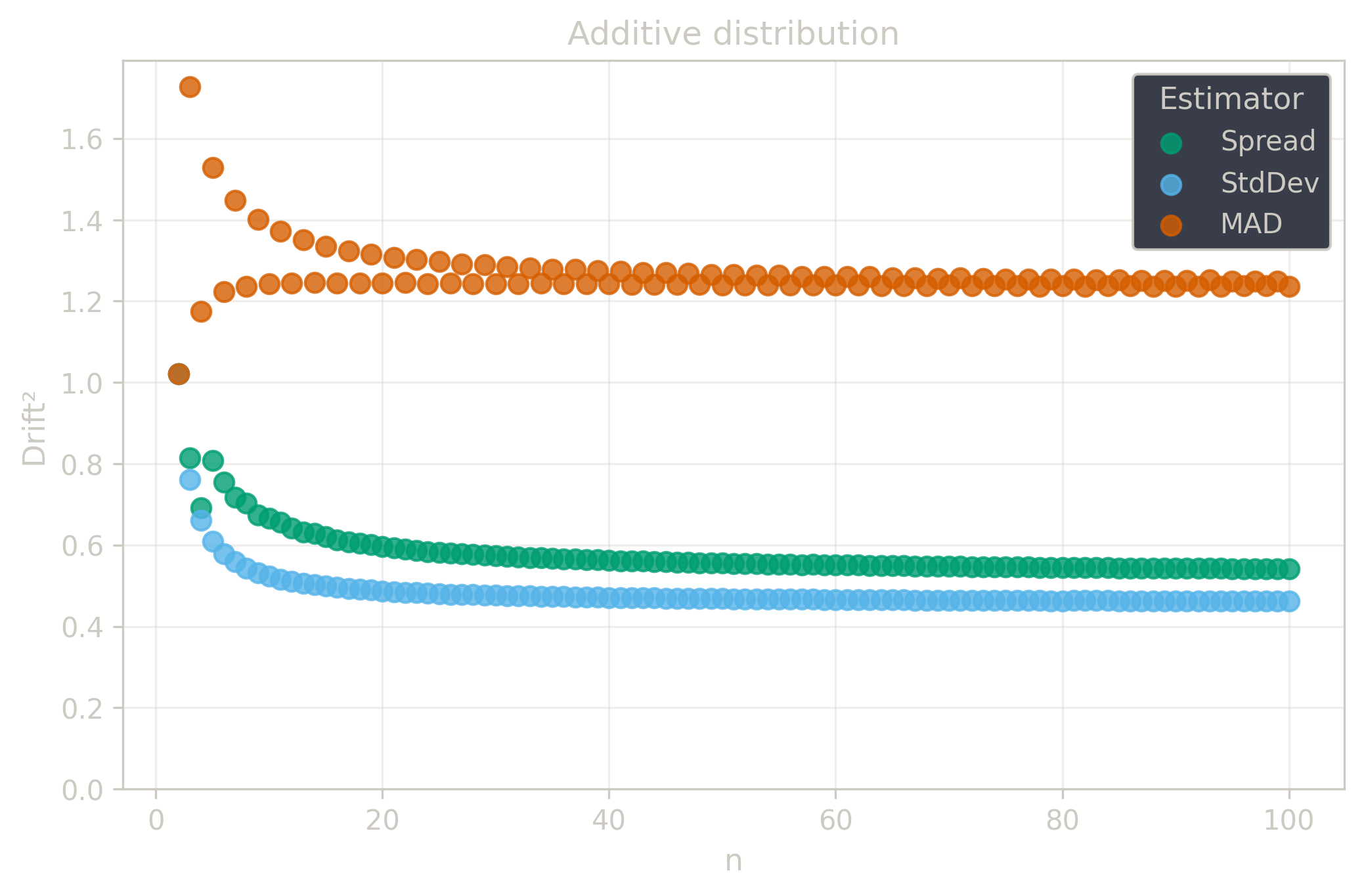
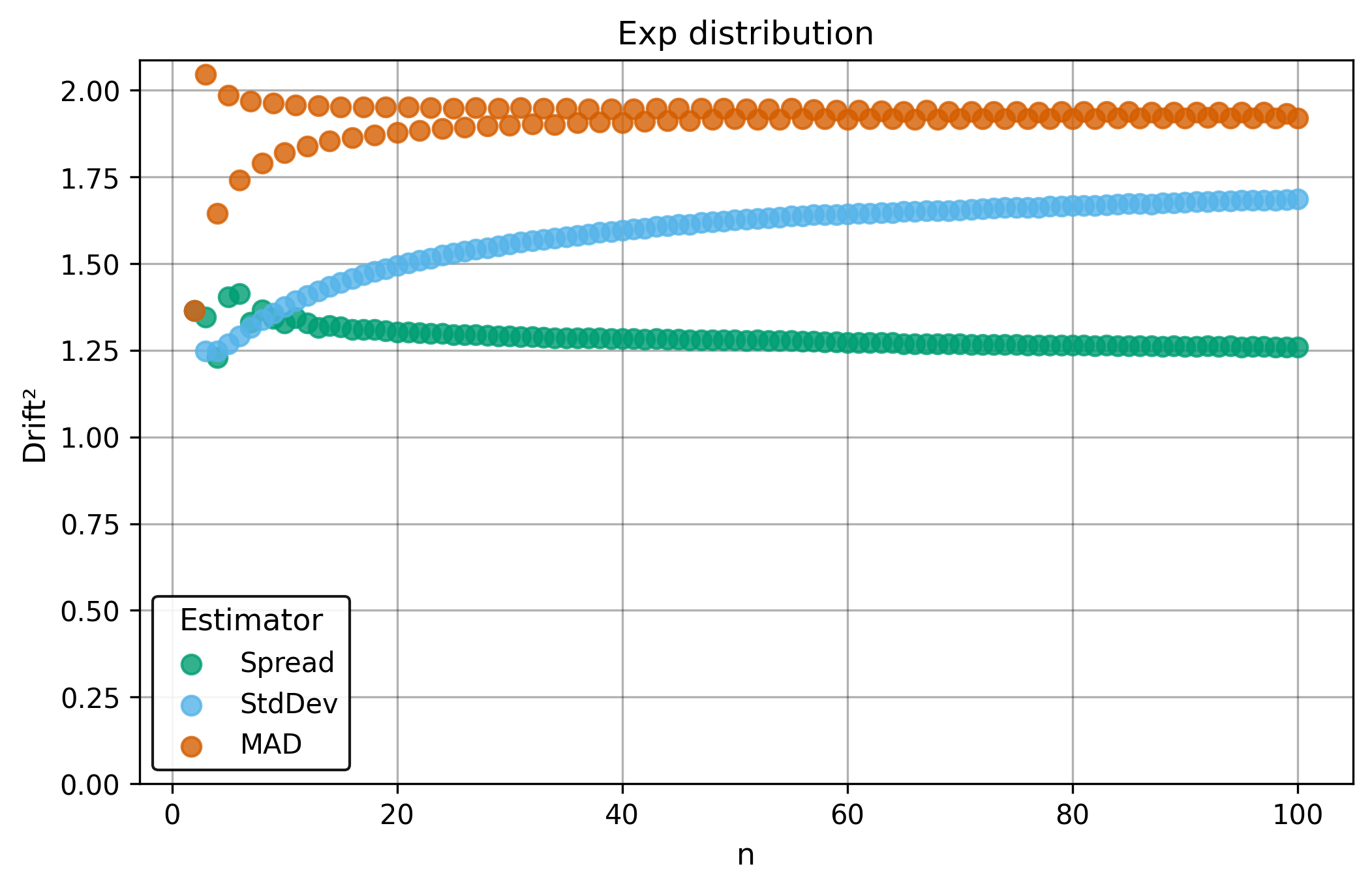
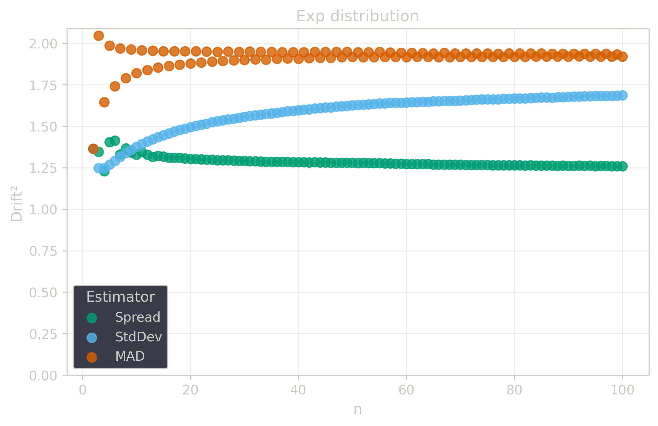
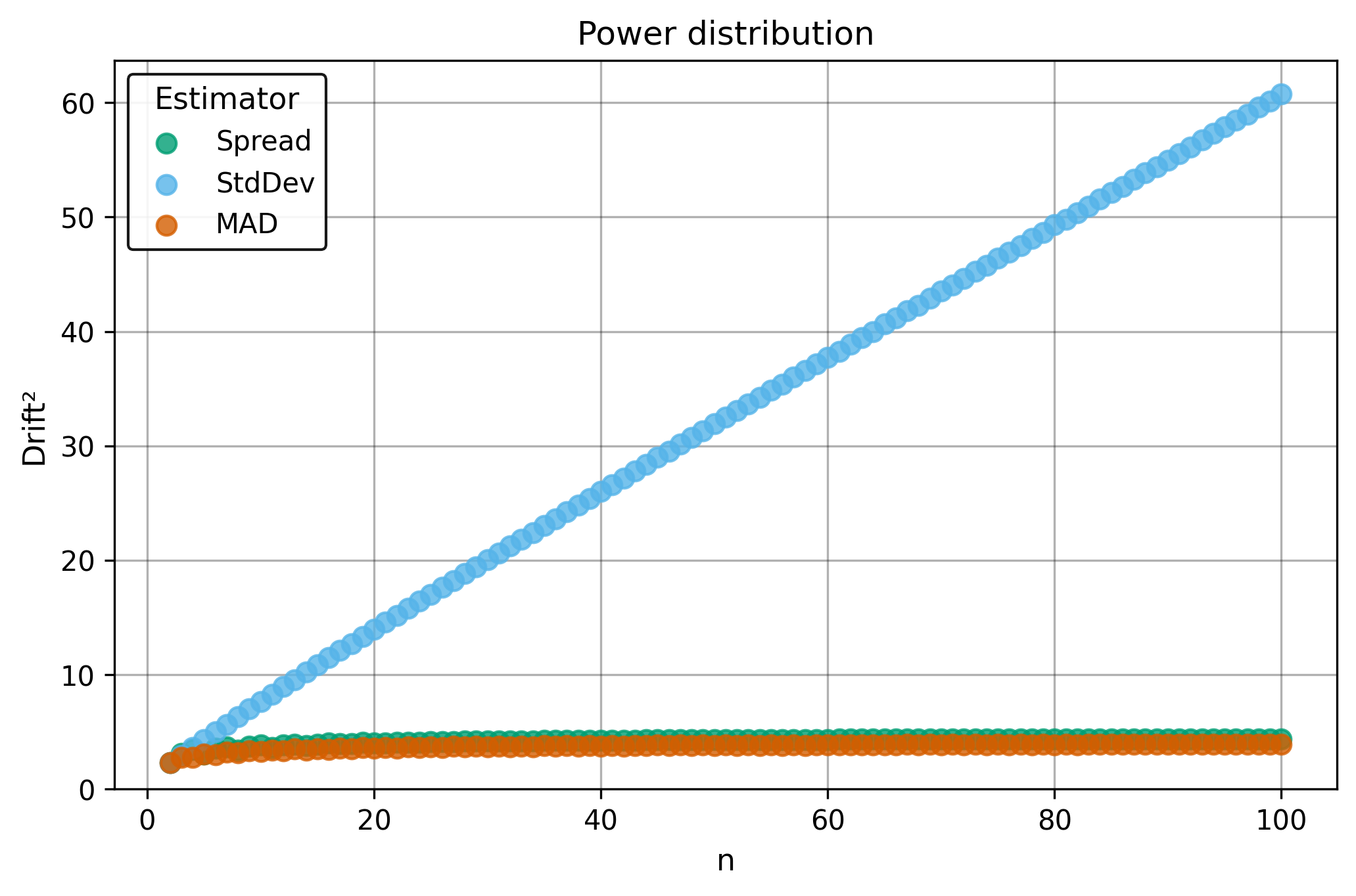
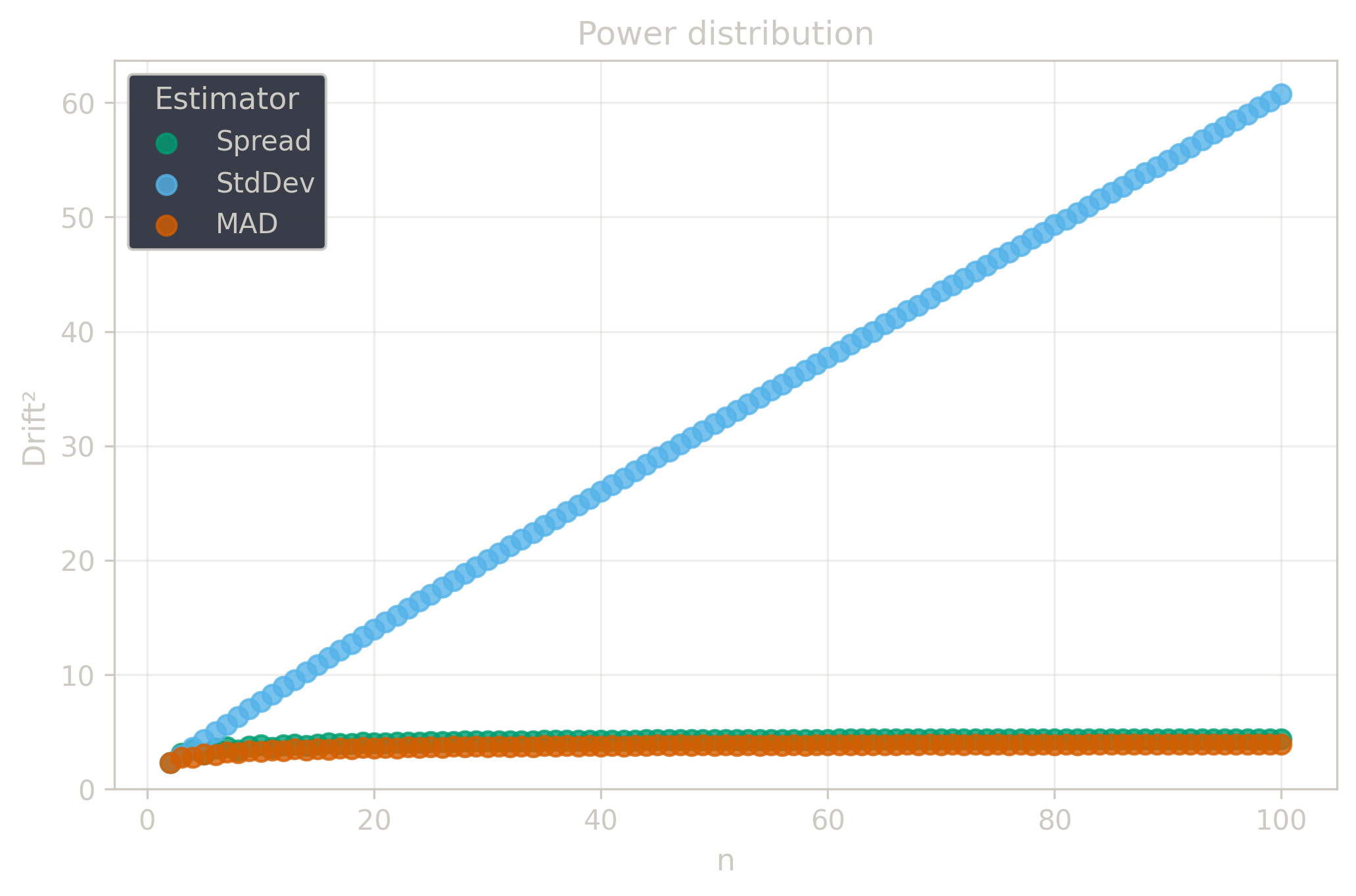
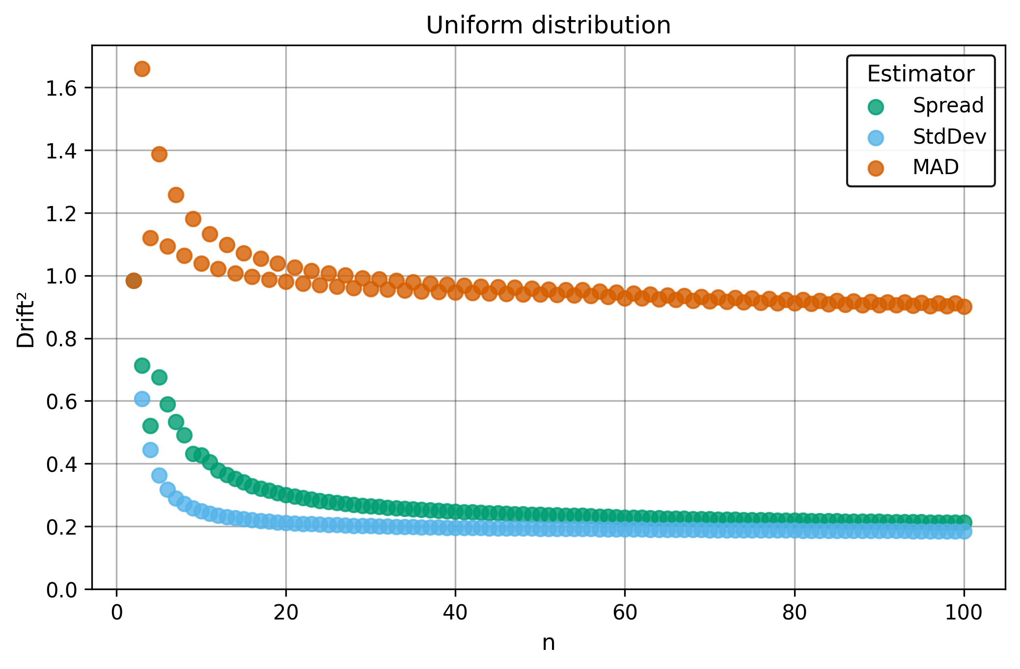
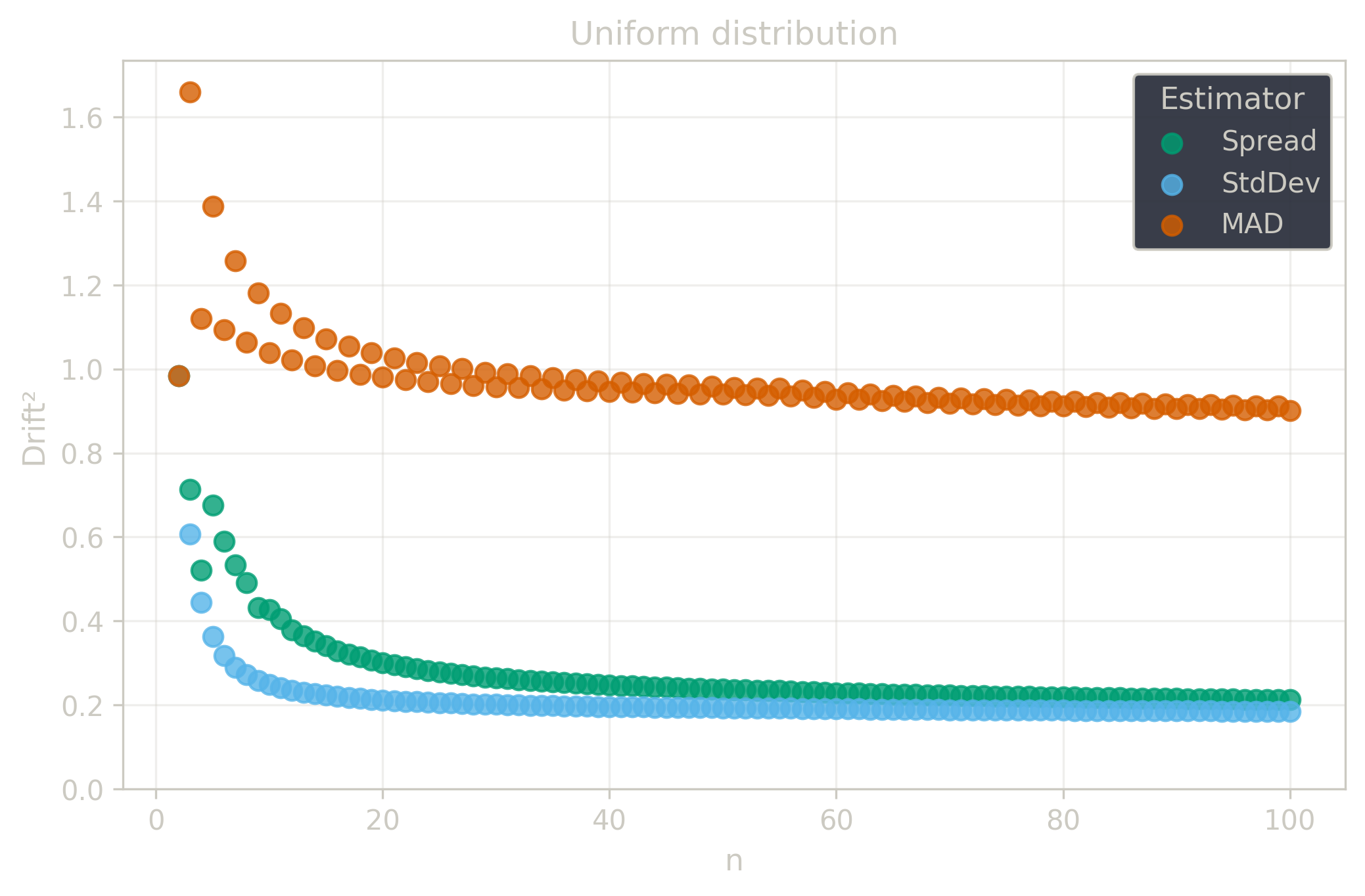
Drift

Drift measures estimator precision by quantifying how much estimates scatter across repeated samples. It is based on the $\operatorname{Spread}$ of estimates and therefore has a breakdown point of approximately $29\%$.

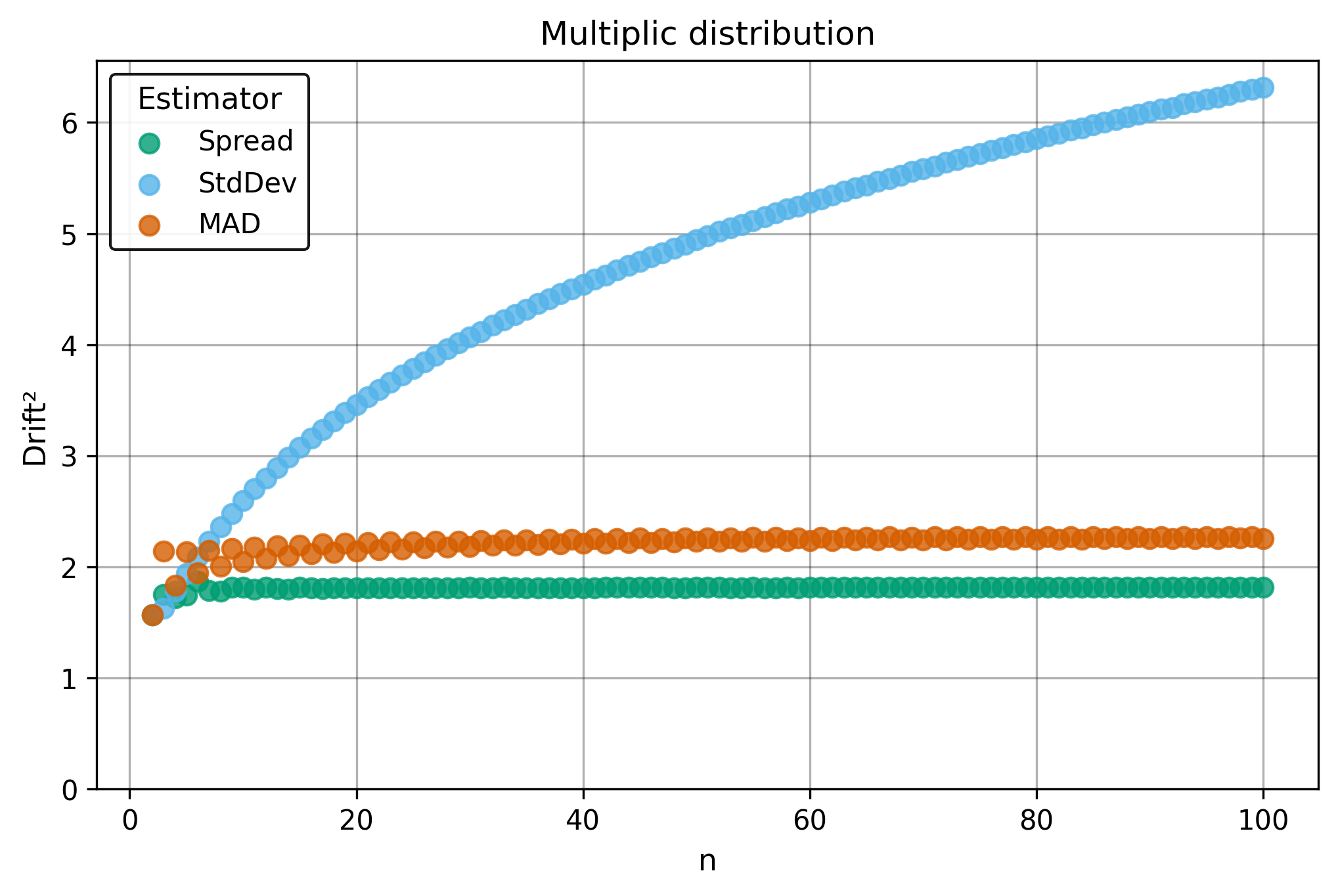
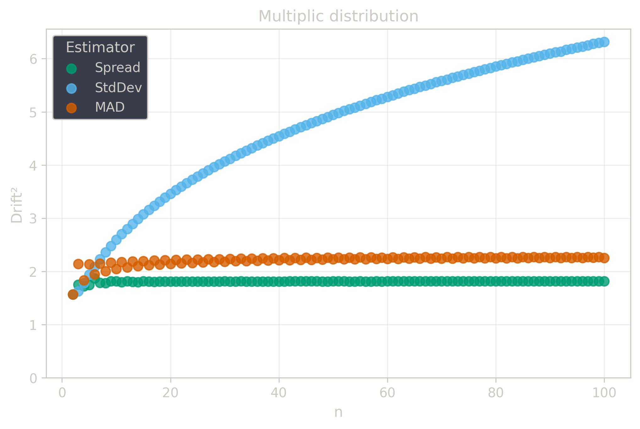
Drift is useful for comparing the precision of several estimators. To simplify the comparison, one of the estimators can be chosen as a baseline. A table of squared drift values, normalized by the baseline, shows the required sample size adjustment factor for switching from the baseline to another estimator. For example, if $\operatorname{Spread}$ is the baseline and the rescaled drift square of $\operatorname{MAD}$ is $1.25$, this means that $\operatorname{MAD}$ requires $1.25$ times more data than $\operatorname{Spread}$ to achieve the same precision. See From Statistical Efficiency to Drift for details.

Squared Asymptotic Drift of Dispersion Estimators (values are approximated):

Rescaled to $\operatorname{Spread}$ (sample size adjustment factors):

Tests

The $\operatorname{Spread}$ test suite contains 30 correctness test cases stored in the repository (20 original + 10 unsorted), plus 1 performance test that should be implemented manually (see Test Framework).

Demo examples ($n = 5$) — from manual introduction, validating properties:

• demo-1: $\mathbf{x} = (0, 2, 4, 6, 8)$, expected output: $4$ (base case)
• demo-2: $\mathbf{x} = (10, 12, 14, 16, 18)$ (= demo-1 + 10), expected output: $4$ (location invariance)
• demo-3: $\mathbf{x} = (0, 4, 8, 12, 16)$ (= 2 × demo-1), expected output: $8$ (scale equivariance)

Natural sequences ($n = 2, 3, 4$):

• natural-2: $\mathbf{x} = (1, 2)$, expected output: $1$
• natural-3: $\mathbf{x} = (1, 2, 3)$, expected output: $1$
• natural-4: $\mathbf{x} = (1, 2, 3, 4)$, expected output: $1.5$ (smallest even size with rich structure)

Negative values ($n = 3$) — sign handling validation:

• negative-3: $\mathbf{x} = (-3, -2, -1)$, expected output: $1$

Additive distribution ($n = 5, 10, 30$) — $\underline{\operatorname{Additive}}(10, 1)$:

• additive-5, additive-10, additive-30: random samples generated with seed 0

Uniform distribution ($n = 5, 100$) — $\underline{\operatorname{Uniform}}(0, 1)$:

• uniform-5, uniform-100: random samples generated with seed 1

The natural sequence cases validate the basic pairwise difference calculation. Constant samples and $n = 1$ are excluded because $\operatorname{Spread}$ requires $\operatorname{Spread}(\mathbf{x}) > 0$.

Algorithm stress tests — edge cases for fast algorithm implementation:

• duplicates-10: $\mathbf{x} = (1, 1, 1, 2, 2, 2, 3, 3, 3, 3)$ (many duplicates, stress tie-breaking)
• parity-odd-7: $\mathbf{x} = (1, 2, 3, 4, 5, 6, 7)$ (odd sample size, 21 differences)
• parity-even-6: $\mathbf{x} = (1, 2, 3, 4, 5, 6)$ (even sample size, 15 differences)
• parity-odd-49: 49-element sequence $(1, 2, \ldots, 49)$ (large odd, 1176 differences)
• parity-even-50: 50-element sequence $(1, 2, \ldots, 50)$ (large even, 1225 differences)

Extreme values — numerical stability and range tests:

• extreme-large-5: $\mathbf{x} = (10^8, 2 \cdot 10^8, 3 \cdot 10^8, 4 \cdot 10^8, 5 \cdot 10^8)$ (very large values)
• extreme-small-5: $\mathbf{x} = (10^{-8}, 2 \cdot 10^{-8}, 3 \cdot 10^{-8}, 4 \cdot 10^{-8}, 5 \cdot 10^{-8})$ (very small positive values)
• extreme-wide-5: $\mathbf{x} = (0.001, 1, 100, 1000, 1000000)$ (wide range, tests precision)

Unsorted tests — verify sorting correctness (10 tests):

• unsorted-reverse-{n} for $n in {2, 3, 4, 5, 7}$: reverse sorted natural sequences (5 tests)
• unsorted-shuffle-3: $\mathbf{x} = (3, 1, 2)$ (rotated)
• unsorted-shuffle-4: $\mathbf{x} = (4, 2, 1, 3)$ (mixed order)
• unsorted-shuffle-5: $\mathbf{x} = (5, 1, 3, 2, 4)$ (partial shuffle)
• unsorted-duplicates-unsorted-10: $\mathbf{x} = (2, 3, 1, 3, 2, 1, 2, 3, 1, 3)$ (duplicates mixed)
• unsorted-extreme-wide-unsorted-5: $\mathbf{x} = (1000, 0.001, 1000000, 100, 1)$ (wide range unsorted)

These tests verify that implementations correctly sort input before computing pairwise differences. Since $\operatorname{Spread}$ uses absolute differences, order-dependent bugs would manifest differently than in $\operatorname{Center}$.

Performance test — validates the fast $O(n \log n)$ algorithm:

• Input: $\mathbf{x} = (1, 2, 3, \ldots, 100000)$
• Expected output: $29290$
• Time constraint: Must complete in under 5 seconds
• Purpose: Ensures that the implementation uses the efficient algorithm rather than materializing all $\binom{n}{2} \approx 5$ billion pairwise differences

This test case is not stored in the repository because it generates a large JSON file (approximately 1.5 MB). Each language implementation should manually implement this test with the hardcoded expected result.

References