Center

Robust measure of location (central tendency).

Input

• $\mathbf{x} = (x_1, x_2, \ldots, x_n)$ — input sample of measurements

Output

• Value — estimation of the median of the average of two random measurements from $X$
• Unit — same unit as $\mathbf{x}$

Notes

• Also known as — Hodges–Lehmann estimator, pseudomedian
• Complexity — $O(n \log n)$

Properties

• Shift equivariance $\operatorname{Center}(\mathbf{x} + k) = \operatorname{Center}(\mathbf{x}) + k$
• Scale equivariance $\operatorname{Center}(k \cdot \mathbf{x}) = k \cdot \operatorname{Center}(\mathbf{x})$

Example

• Center([0, 2, 4, 6, 8]) = 4
• Center(x + 10) = 14 Center(3x) = 12

$\operatorname{Center}$ is the recommended default for representing “where the data is.” It works like the familiar mean but does not break when the data contains a few bad measurements or outliers. Up to 29% of data can be corrupted before $\operatorname{Center}$ becomes unreliable. When data is clean, $\operatorname{Center}$ is nearly as precise as the mean (95% efficiency), so the added protection comes at almost no cost. When uncertain whether to use mean, median, or something else, start with $\operatorname{Center}$.

Algorithm

The $\operatorname{Center}$ estimator computes the median of all pairwise averages from a sample. Given a dataset $x = (x_1, x_2, \ldots, x_n)$, this estimator is defined as:

A direct implementation would generate all $n(n+1)/2$ pairwise averages and sort them. With $n = 10000$, this approach creates approximately 50 million values, requiring quadratic memory and $O(n^2 \log n)$ time.

The breakthrough came in 1984 when John Monahan developed an algorithm that reduces expected complexity to $O(n \log n)$ while using only linear memory (see Monahan 1984). The algorithm exploits the inherent structure in pairwise sums rather than computing them explicitly. After sorting the values $x_1 \leq x_2 \leq \ldots \leq x_n$, the algorithm considers the implicit upper triangular matrix $M$ where $M_{i,j} = x_i + x_j$ for $i \leq j$. This matrix has a crucial property: each row and column is sorted in non-decreasing order, enabling efficient median selection without storing the matrix.

Rather than sorting all pairwise sums, the algorithm uses a selection approach similar to quickselect. It maintains search bounds for each matrix row and iteratively narrows the search space. For each row $i$, the algorithm tracks active column indices from $i+1$ to $n$, defining which pairwise sums remain candidates for the median. It selects a candidate sum as a pivot using randomized selection from active matrix elements, then counts how many pairwise sums fall below the pivot. Because both rows and columns are sorted, this counting takes only $O(n)$ time using a two-pointer sweep from the matrix’s upper-right corner.

The median corresponds to rank $k = \lfloor (N+1)/2 \rfloor$ where $N = n(n+1)/2$. If fewer than $k$ sums lie below the pivot, the median must be larger; if more than $k$ sums lie below the pivot, the median must be smaller. Based on this comparison, the algorithm eliminates portions of each row that cannot contain the median, shrinking the active search space while preserving the true median.

Real data often contain repeated values, which can cause the selection process to stall. When the algorithm detects no progress between iterations, it switches to a midrange strategy: find the smallest and largest pairwise sums still in the search space, then use their average as the next pivot. If the minimum equals the maximum, all remaining candidates are identical and the algorithm terminates. This tie-breaking mechanism ensures reliable convergence with discrete or duplicated data.

The algorithm achieves $O(n \log n)$ time complexity through linear partitioning (each pivot evaluation requires only $O(n)$ operations) and logarithmic iterations (randomized pivot selection leads to expected $O(\log n)$ iterations, similar to quickselect). The algorithm maintains only row bounds and counters, using $O(n)$ additional space. This matches the complexity of sorting a single array while avoiding the quadratic memory and time explosion of computing all pairwise combinations.

using Pragmastat.Internal;
using Pragmastat.Randomization;

namespace Pragmastat.Algorithms;

internal static class CenterImpl
{
  // Bound the selection loop. On valid sorted input the Monahan selection converges in
  // O(log n) iterations; the cap (BaseIterations + 4 * n) is far higher than ever needed for
  // sorted input but guarantees termination on misuse (e.g. assumeSorted=true on UNSORTED
  // input, which is undefined behavior and would otherwise spin forever). The cap scales with
  // n so large valid inputs are never starved. We also track no-progress (stall) on the
  // active set to bail out deterministically.
  private const int BaseIterations = 256;
  private const int MaxStall = 8;
  /// <summary>
  /// ACM Algorithm 616: fast computation of the Hodges-Lehmann location estimator
  /// </summary>
  /// <remarks>
  /// Computes the median of all pairwise averages (xi + xj)/2 efficiently.
  /// See: John F Monahan, "Algorithm 616: fast computation of the Hodges-Lehmann location estimator"
  /// (1984) DOI: 10.1145/1271.319414
  /// </remarks>
  /// <param name="values">Sample values; sorted only when assumeSorted is true</param>
  /// <param name="assumeSorted">If values are sorted</param>
  /// <returns>Exact center value (Hodges-Lehmann estimator)</returns>
  public static double Estimate(IReadOnlyList<double> values, bool assumeSorted = false)
  {
    int n = values.Count;
    if (n == 1) return values[0];
    // Overflow-safe, order-symmetric midpoint: 0.5*a + 0.5*b (halve before summing;
    // never overflows; operand order is irrelevant).
    if (n == 2) return Midpoint(values[0], values[1]);
    // Deterministic RNG seeded from the input (FNV-1a), matching the other languages.
    var rng = new Rng((long)Fnv1a.HashDoubles(values));
    if (!assumeSorted)
      values = values.CopyToArrayAndSort();

    // Calculate target median rank(s) among all pairwise sums
    long totalPairs = (long)n * (n + 1) / 2;
    long medianRankLow = (totalPairs + 1) / 2; // For odd totalPairs, this is the median
    long medianRankHigh =
      (totalPairs + 2) / 2; // For even totalPairs, average of ranks medianRankLow and medianRankHigh

    // Initialize search bounds for each row in the implicit matrix
    long[] leftBounds = new long[n];
    long[] rightBounds = new long[n];
    long[] partitionCounts = new long[n];

    for (int i = 0; i < n; i++)
    {
      leftBounds[i] = i + 1; // Row i can pair with columns [i+1..n] (1-based indexing)
      rightBounds[i] = n; // Initially, all columns are available
    }

    // Start with a good pivot: sum of middle elements (handles both odd and even n)
    double pivot = values[(n - 1) / 2] + values[n / 2];
    long activeSetSize = totalPairs;
    long previousCount = 0;

    int maxIterations = BaseIterations + 4 * n;
    long prevActiveSetSize = -1;
    int stallCount = 0;

    for (int iter = 0; iter < maxIterations; iter++)
    {
      // === PARTITION STEP ===
      // Count pairwise sums less than current pivot
      long countBelowPivot = 0;
      long currentColumn = n;

      for (int row = 1; row <= n; row++)
      {
        partitionCounts[row - 1] = 0;

        // Move left from current column until we find sums < pivot
        // This exploits the sorted nature of the matrix
        while (currentColumn >= row && values[row - 1] + values[(int)currentColumn - 1] >= pivot)
          currentColumn--;

        // Count elements in this row that are < pivot
        if (currentColumn >= row)
        {
          long elementsBelow = currentColumn - row + 1;
          partitionCounts[row - 1] = elementsBelow;
          countBelowPivot += elementsBelow;
        }
      }

      // === CONVERGENCE CHECK ===
      // If no progress, we have ties - break them using midrange strategy
      if (countBelowPivot == previousCount)
      {
        double minActiveSum = double.MaxValue;
        double maxActiveSum = double.MinValue;

        // Find the range of sums still in the active search space
        for (int i = 0; i < n; i++)
        {
          if (leftBounds[i] > rightBounds[i]) continue; // Skip empty rows

          double rowValue = values[i];
          double smallestInRow = values[(int)leftBounds[i] - 1] + rowValue;
          double largestInRow = values[(int)rightBounds[i] - 1] + rowValue;

          minActiveSum = Min(minActiveSum, smallestInRow);
          maxActiveSum = Max(maxActiveSum, largestInRow);
        }

        pivot = 0.5 * minActiveSum + 0.5 * maxActiveSum;
        if (pivot <= minActiveSum || pivot > maxActiveSum) pivot = maxActiveSum;

        // If all remaining values are identical, we're done
        if (minActiveSum == maxActiveSum || activeSetSize <= 2)
          return pivot / 2;

        continue;
      }

      // === TARGET CHECK ===
      // Check if we've found the median rank(s)
      bool atTargetRank = countBelowPivot == medianRankLow || countBelowPivot == medianRankHigh - 1;
      if (atTargetRank)
      {
        // Find the boundary values: largest < pivot and smallest >= pivot
        double largestBelowPivot = double.MinValue;
        double smallestAtOrAbovePivot = double.MaxValue;

        for (int i = 1; i <= n; i++)
        {
          long countInRow = partitionCounts[i - 1];
          double rowValue = values[i - 1];
          long totalInRow = n - i + 1;

          // Find largest sum in this row that's < pivot
          if (countInRow > 0)
          {
            long lastBelowIndex = i + countInRow - 1;
            double lastBelowValue = rowValue + values[(int)lastBelowIndex - 1];
            largestBelowPivot = Max(largestBelowPivot, lastBelowValue);
          }

          // Find smallest sum in this row that's >= pivot
          if (countInRow < totalInRow)
          {
            long firstAtOrAboveIndex = i + countInRow;
            double firstAtOrAboveValue = rowValue + values[(int)firstAtOrAboveIndex - 1];
            smallestAtOrAbovePivot = Min(smallestAtOrAbovePivot, firstAtOrAboveValue);
          }
        }

        // Calculate final result based on whether we have odd or even number of pairs
        if (medianRankLow < medianRankHigh)
        {
          // Even total: average the two middle values. Overflow-safe: quarter each
          // pair-sum before summing (both operands can be near the double max).
          return 0.25 * smallestAtOrAbovePivot + 0.25 * largestBelowPivot;
        }
        else
        {
          // Odd total: return the single middle value
          bool needLargest = countBelowPivot == medianRankLow;
          return (needLargest ? largestBelowPivot : smallestAtOrAbovePivot) / 2;
        }
      }

      // === UPDATE BOUNDS ===
      // Narrow the search space based on partition result
      if (countBelowPivot < medianRankLow)
      {
        // Too few values below pivot - eliminate smaller values, search higher
        for (int i = 0; i < n; i++)
          leftBounds[i] = i + partitionCounts[i] + 1;
      }
      else
      {
        // Too many values below pivot - eliminate larger values, search lower
        for (int i = 0; i < n; i++)
          rightBounds[i] = i + partitionCounts[i];
      }

      // === PREPARE NEXT ITERATION ===
      previousCount = countBelowPivot;

      // Recalculate how many elements remain in the active search space
      activeSetSize = 0;
      for (int i = 0; i < n; i++)
      {
        long rowSize = rightBounds[i] - leftBounds[i] + 1;
        activeSetSize += Max(0, rowSize);
      }

      // Stall detection: on valid sorted input the active set strictly shrinks toward the
      // target. If it fails to shrink for several consecutive iterations, the input is
      // pathological (e.g. assumeSorted=true on unsorted data) and we bail deterministically.
      if (activeSetSize >= prevActiveSetSize && prevActiveSetSize >= 0)
      {
        stallCount++;
        if (stallCount >= MaxStall)
          throw new InvalidOperationException("Convergence failure (pathological input).");
      }
      else
      {
        stallCount = 0;
      }

      prevActiveSetSize = activeSetSize;

      // Choose next pivot based on remaining active set size
      if (activeSetSize > 2)
      {
        // Use randomized row median strategy for efficiency
        long targetIndex = rng.UniformInt64(0, activeSetSize);
        int selectedRow = 0;

        // Find which row contains the target index
        long cumulativeSize = 0;
        for (int i = 0; i < n; i++)
        {
          long rowSize = Max(0, rightBounds[i] - leftBounds[i] + 1);
          if (targetIndex < cumulativeSize + rowSize)
          {
            selectedRow = i;
            break;
          }

          cumulativeSize += rowSize;
        }

        // Use median element of the selected row as pivot
        long medianColumnInRow = (leftBounds[selectedRow] + rightBounds[selectedRow]) / 2;
        pivot = values[selectedRow] + values[(int)medianColumnInRow - 1];
      }
      else
      {
        // Few elements remain - use midrange strategy
        double minRemainingSum = double.MaxValue;
        double maxRemainingSum = double.MinValue;

        for (int i = 0; i < n; i++)
        {
          if (leftBounds[i] > rightBounds[i]) continue; // Skip empty rows

          double rowValue = values[i];
          double minInRow = values[(int)leftBounds[i] - 1] + rowValue;
          double maxInRow = values[(int)rightBounds[i] - 1] + rowValue;

          minRemainingSum = Min(minRemainingSum, minInRow);
          maxRemainingSum = Max(maxRemainingSum, maxInRow);
        }

        pivot = 0.5 * minRemainingSum + 0.5 * maxRemainingSum;
        if (pivot <= minRemainingSum || pivot > maxRemainingSum)
          pivot = maxRemainingSum;

        if (minRemainingSum == maxRemainingSum)
          return pivot / 2;
      }
    }

    // Iteration cap exhausted. The selection loop converges in O(log n) iterations on valid
    // sorted input, so reaching here means the contract was violated (e.g. assumeSorted=true
    // on unsorted input). Fail deterministically instead of spinning forever. Plain exception
    // (NOT an AssumptionException): this is a misuse/pathological-input guard.
    throw new InvalidOperationException("Convergence failure (pathological input).");
  }

  // Overflow-safe, order-symmetric midpoint: 0.5*a + 0.5*b (halve before summing;
  // never overflows; operand order is irrelevant).
  private static double Midpoint(double a, double b) => 0.5 * a + 0.5 * b;
}

Notes

This section compares the toolkit’s robust average estimator against traditional methods to demonstrate its advantages across diverse conditions.

Average Estimators

Mean (arithmetic average):

Median:

Center (Hodges–Lehmann estimator):

Breakdown

Heavy-tailed distributions naturally produce extreme outliers that completely distort traditional estimators. A single extreme measurement from the $\underline{\operatorname{Power}}$ distribution can make the sample mean arbitrarily large. Real-world data can also contain corrupted measurements from instrument failures, recording errors, or transmission problems. Both natural extremes and data corruption create the same challenge: extracting reliable information when some measurements are too influential.

The breakdown point (Huber 2009) is the fraction of a sample that can be replaced by arbitrarily large values without making an estimator arbitrarily large. The theoretical maximum is $50\%$; no estimator can guarantee reliable results when more than half the measurements are extreme or corrupted. In such cases, summary estimators are not applicable, and a more sophisticated approach is needed.

A $50\%$ breakdown point is rarely needed in practice, as more conservative values also cover practical needs. Additionally, a high breakdown point corresponds to low precision (information is lost by neglecting part of the data). The optimal practical breakdown point should be between $0\%$ (no robustness) and $50\%$ (low precision).

The $\operatorname{Center}$ estimator achieves a $29\%$ breakdown point, providing substantial protection against realistic contamination levels while maintaining good precision.

Asymptotic breakdown points for average estimators:

Drift

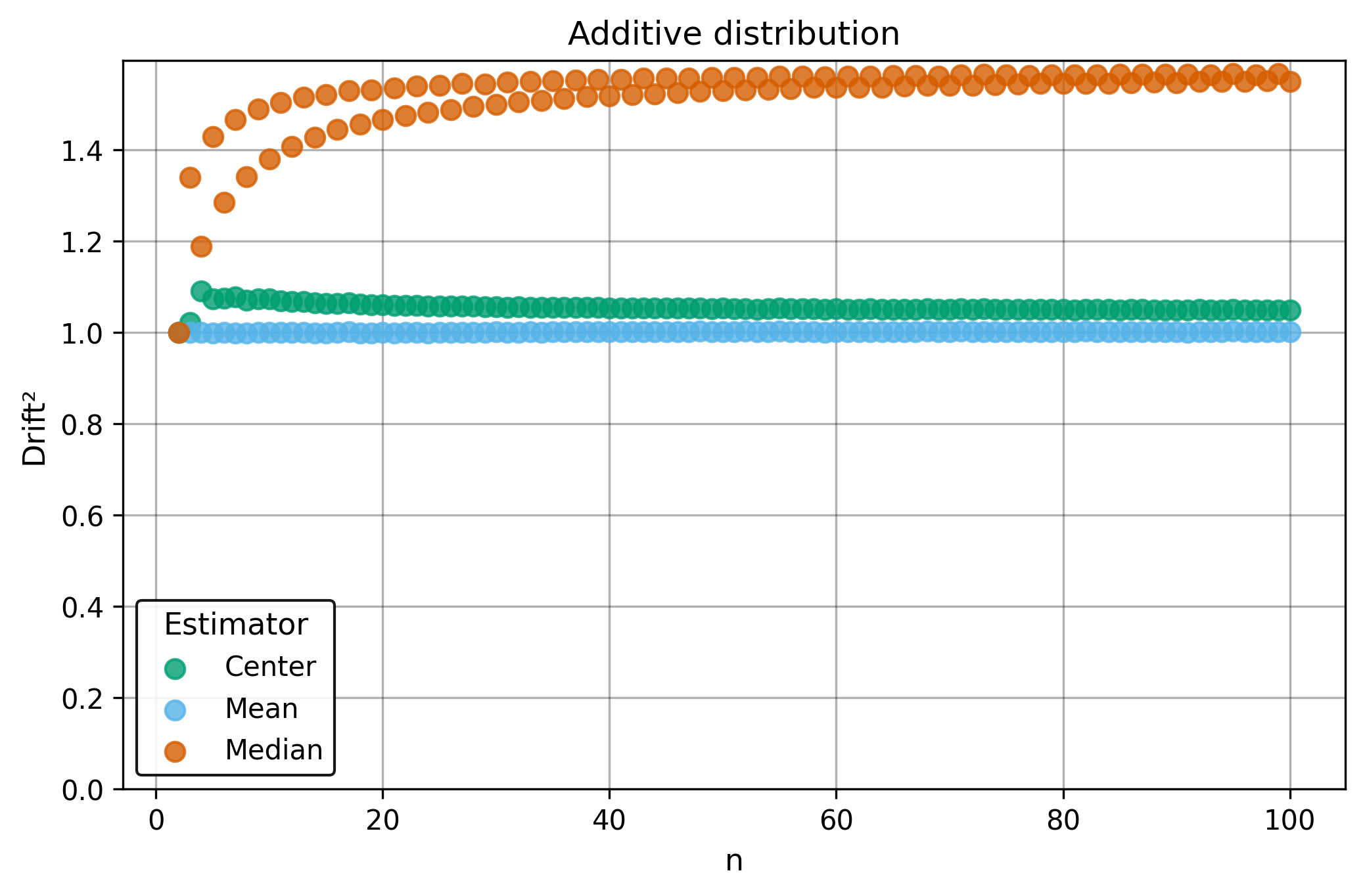
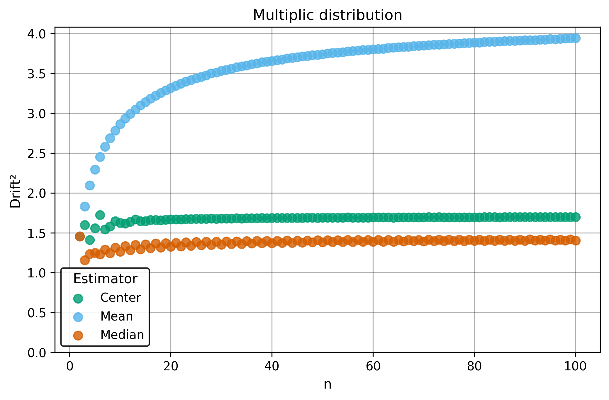
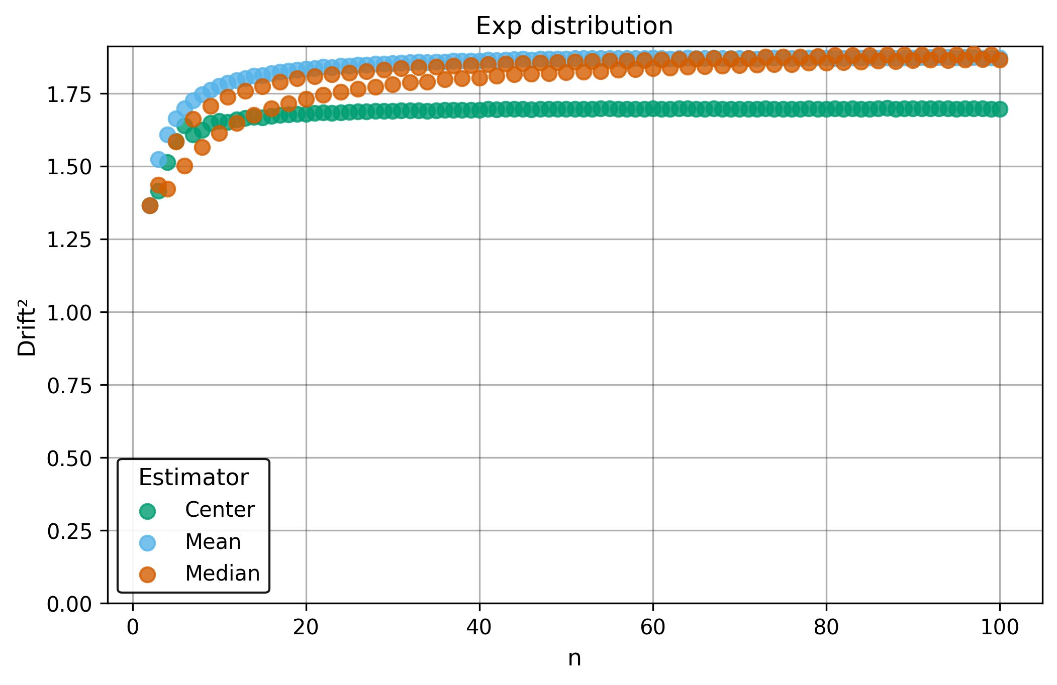
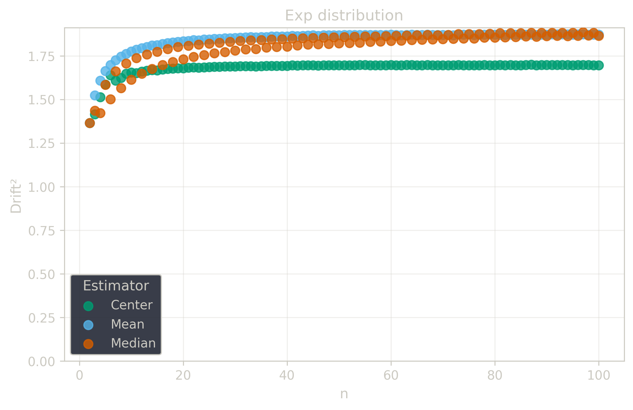
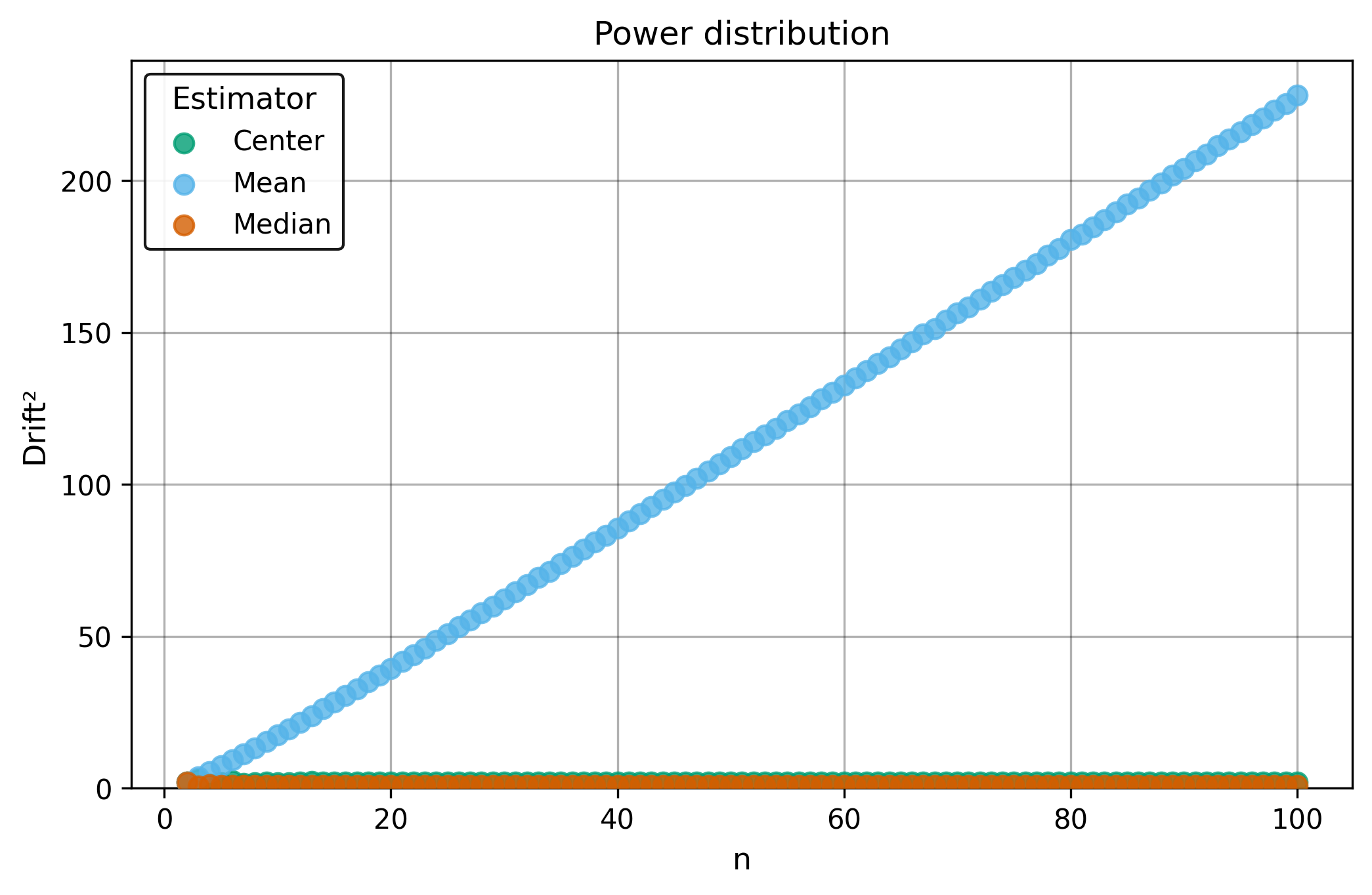
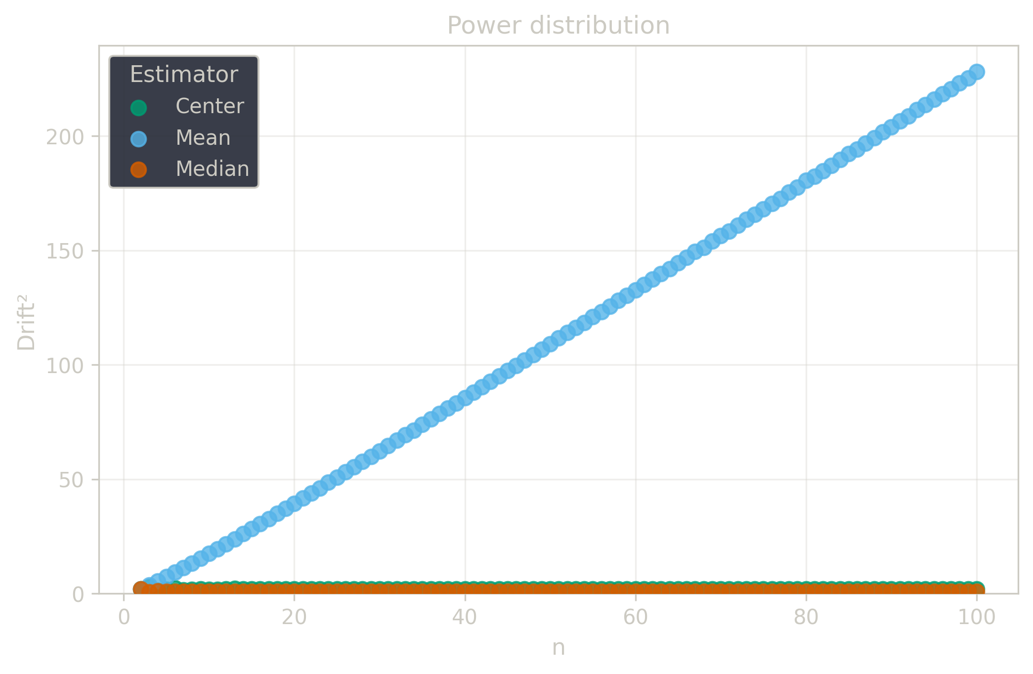
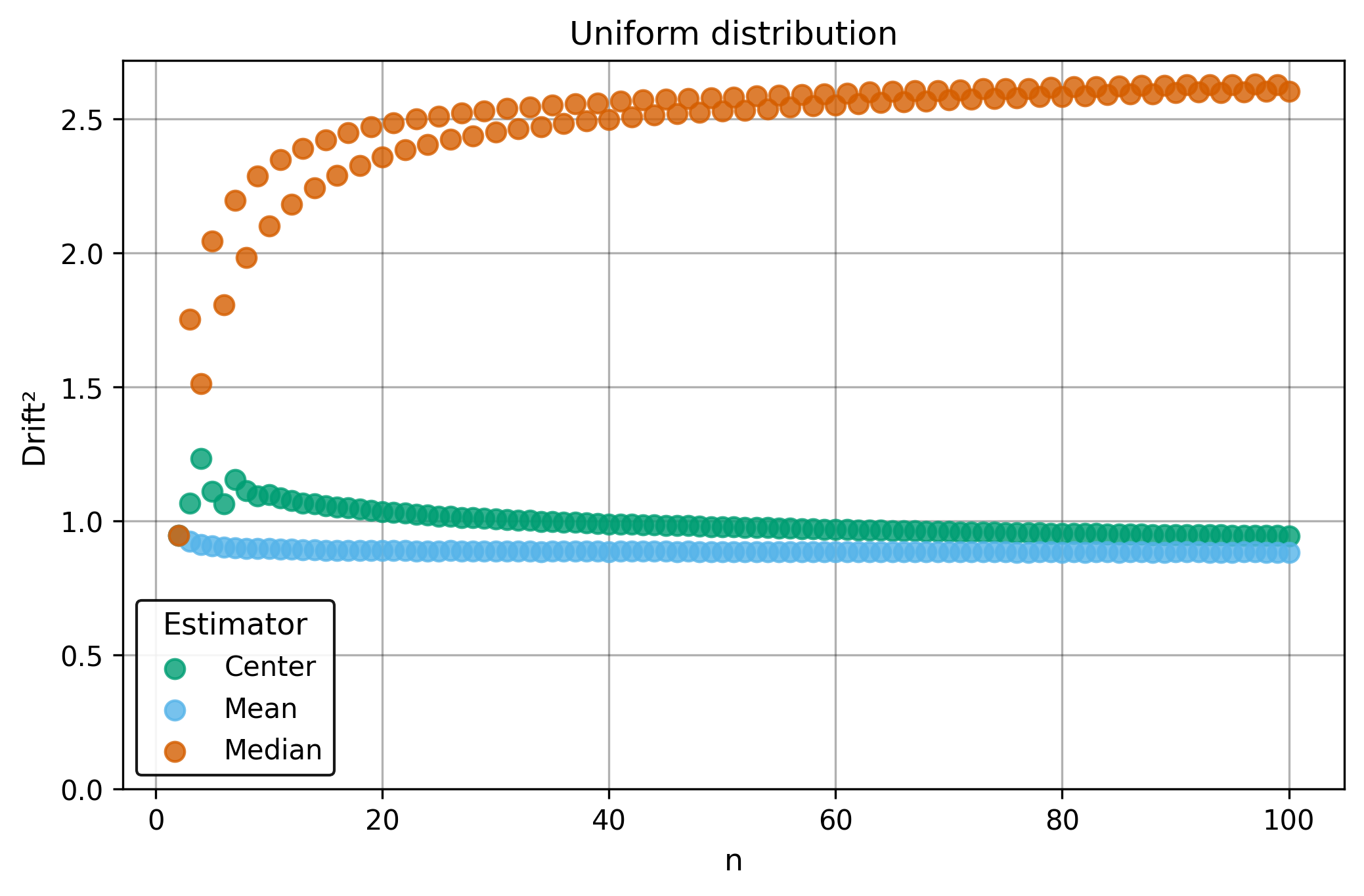
Drift measures estimator precision by quantifying how much estimates scatter across repeated samples. It is based on the $\operatorname{Spread}$ of estimates, so its empirical evaluation across repeated samples inherits the $29\%$ breakdown point of $\operatorname{Spread}$.

Drift is useful for comparing the precision of several estimators. To simplify the comparison, one of the estimators can be chosen as a baseline. A table of squared drift values, normalized by the baseline, shows the required sample size adjustment factor for switching from the baseline to another estimator. For example, if $\operatorname{Center}$ is the baseline and the rescaled drift square of $\operatorname{Median}$ is $1.5$, this means that $\operatorname{Median}$ requires $1.5$ times more data than $\operatorname{Center}$ to achieve the same precision. See From Statistical Efficiency to Drift for details.

Squared Asymptotic Drift of Average Estimators (values are approximated):

Rescaled to $\operatorname{Center}$ (sample size adjustment factors):

Tests

The $\operatorname{Center}$ test suite contains 43 test cases stored in the repository (28 original + 14 unsorted + 1 error), plus 1 performance test that should be implemented manually (see Test Framework).

Demo examples ($n = 5$) — from manual introduction, validating properties:

• demo-1: $\mathbf{x} = (0, 2, 4, 6, 8)$, expected output: $4$ (base case)
• demo-2: $\mathbf{x} = (10, 12, 14, 16, 18)$ (= demo-1 + 10), expected output: $14$ (location equivariance)
• demo-3: $\mathbf{x} = (0, 6, 12, 18, 24)$ (= 3 × demo-1), expected output: $12$ (scale equivariance)

Natural sequences ($n = 1, 2, 3, 4$) — canonical happy path examples:

• natural-1: $\mathbf{x} = (1)$, expected output: $1$
• natural-2: $\mathbf{x} = (1, 2)$, expected output: $1.5$
• natural-3: $\mathbf{x} = (1, 2, 3)$, expected output: $2$
• natural-4: $\mathbf{x} = (1, 2, 3, 4)$, expected output: $2.5$ (smallest even size with rich structure)

Negative values ($n = 3$) — sign handling validation:

• negative-3: $\mathbf{x} = (-3, -2, -1)$, expected output: $-2$

Zero values ($n = 1, 2$) — edge case testing with zeros:

• zeros-1: $\mathbf{x} = (0)$, expected output: $0$
• zeros-2: $\mathbf{x} = (0, 0)$, expected output: $0$

Additive distribution ($n = 5, 10, 30$) — fuzzy testing with $\underline{\operatorname{Additive}}(10, 1)$:

• additive-5, additive-10, additive-30: random samples generated with seed 0

Uniform distribution ($n = 5, 100$) — fuzzy testing with $\underline{\operatorname{Uniform}}(0, 1)$:

• uniform-5, uniform-100: random samples generated with seed 1

The random samples validate that $\operatorname{Center}$ performs correctly on realistic distributions at various sample sizes. The progression from small ($n = 5$) to large ($n = 100$) samples helps identify issues that only manifest at specific scales.

Algorithm stress tests — edge cases for the $O(n \log n)$ implementation:

• duplicates-5: $\mathbf{x} = (3, 3, 3, 3, 3)$ (all identical, stress stall handling)
• duplicates-10: $\mathbf{x} = (1, 1, 1, 2, 2, 2, 3, 3, 3, 3)$ (many duplicates, stress tie-breaking)
• parity-odd-7: $\mathbf{x} = (1, 2, 3, 4, 5, 6, 7)$ (odd sample size for odd total pairs)
• parity-even-6: $\mathbf{x} = (1, 2, 3, 4, 5, 6)$ (even sample size for even total pairs)
• parity-odd-49: 49-element sequence $(1, 2, \ldots, 49)$ (large odd, 1225 pairs)
• parity-even-50: 50-element sequence $(1, 2, \ldots, 50)$ (large even, 1275 pairs)

Extreme values — numerical stability and range tests:

• extreme-large-5: $\mathbf{x} = (10^8, 2 \cdot 10^8, 3 \cdot 10^8, 4 \cdot 10^8, 5 \cdot 10^8)$ (very large values)
• extreme-small-5: $\mathbf{x} = (10^{-8}, 2 \cdot 10^{-8}, 3 \cdot 10^{-8}, 4 \cdot 10^{-8}, 5 \cdot 10^{-8})$ (very small positive values)
• extreme-wide-5: $\mathbf{x} = (0.001, 1, 100, 1000, 1000000)$ (wide range, tests precision)
• large-magnitude-2: $\mathbf{x} = (10^308, 10^308)$, expected output: $10^308$ (overflow-safe midpoint: $0.5 x_i + 0.5 x_j$ avoids the $x_i + x_j$ overflow to infinity)
• large-magnitude-negative-2: $\mathbf{x} = (-10^308, -10^308)$, expected output: $-10^308$ (negative-magnitude counterpart)
• opposite-extreme-2: $\mathbf{x} = (-10^308, 10^308)$, expected output: $0$ (opposite extremes cancel without overflow)
• large-magnitude-3: $\mathbf{x} = (8 \cdot 10^307, 8.5 \cdot 10^307, 8.9 \cdot 10^307)$, expected output: $8.475 \cdot 10^307$ (even pair total: the two central pair-sums are finite but overflow when added, so the final average must be computed as $0.25 A + 0.25 B$)

Unsorted tests — verify sorting correctness (14 tests):

• unsorted-reverse-{n} for $n in {2, 3, 4, 5, 7}$: reverse sorted natural sequences (5 tests)
• unsorted-shuffle-3: $\mathbf{x} = (2, 1, 3)$ (middle element first)
• unsorted-shuffle-4: $\mathbf{x} = (3, 1, 4, 2)$ (interleaved)
• unsorted-shuffle-5: $\mathbf{x} = (5, 2, 4, 1, 3)$ (complex shuffle)
• unsorted-last-first-5: $\mathbf{x} = (5, 1, 2, 3, 4)$ (last moved to first)
• unsorted-first-last-5: $\mathbf{x} = (2, 3, 4, 5, 1)$ (first moved to last)
• unsorted-duplicates-mixed-5: $\mathbf{x} = (3, 3, 3, 3, 3)$ (all identical, any order)
• unsorted-duplicates-unsorted-10: $\mathbf{x} = (3, 1, 2, 3, 1, 3, 2, 1, 3, 2)$ (duplicates mixed)
• unsorted-extreme-large-unsorted-5: $\mathbf{x} = (5 \cdot 10^8, 10^8, 4 \cdot 10^8, 2 \cdot 10^8, 3 \cdot 10^8)$ (large values unsorted)
• unsorted-parity-odd-reverse-7: $\mathbf{x} = (7, 6, 5, 4, 3, 2, 1)$ (odd size reverse)

These tests ensure implementations correctly sort input data before computing pairwise averages. The variety of shuffle patterns (reverse, rotation, interleaving, single element displacement) catches common sorting bugs.

Error case — input validation:

• error-empty-x: $\mathbf{x} = ()$ — empty array violates validity

Performance test — validates the $O(n \log n)$ algorithm:

• Input: $\mathbf{x} = (1, 2, 3, \ldots, 100000)$
• Expected output: $50000.5$
• Time constraint: Must complete in under 5 seconds
• Purpose: Ensures that the implementation uses the efficient algorithm rather than materializing all $\binom{n+1}{2} \approx 5$ billion pairwise averages

This test case is not stored in the repository because it generates a large JSON file (approximately 1.5 MB). Each language implementation should manually implement this test with the hardcoded expected result.

References