Additive

• $\mathrm{mean}$: location parameter (center of the distribution), consistent with $\operatorname{Center}$
• $\mathrm{stdDev}$: scale parameter (standard deviation), can be rescaled to $\operatorname{Spread}$

• Formation: the sum of many variables $X_1 + X_2 + \ldots + X_n$ under mild CLT (Central Limit Theorem) conditions (e.g., Lindeberg-Feller).
• Origin: historically called Normal or Gaussian distribution after Carl Friedrich Gauss and others.
• Rename Motivation: renamed to $\underline{\operatorname{Additive}}$ to reflect its formation mechanism through addition.
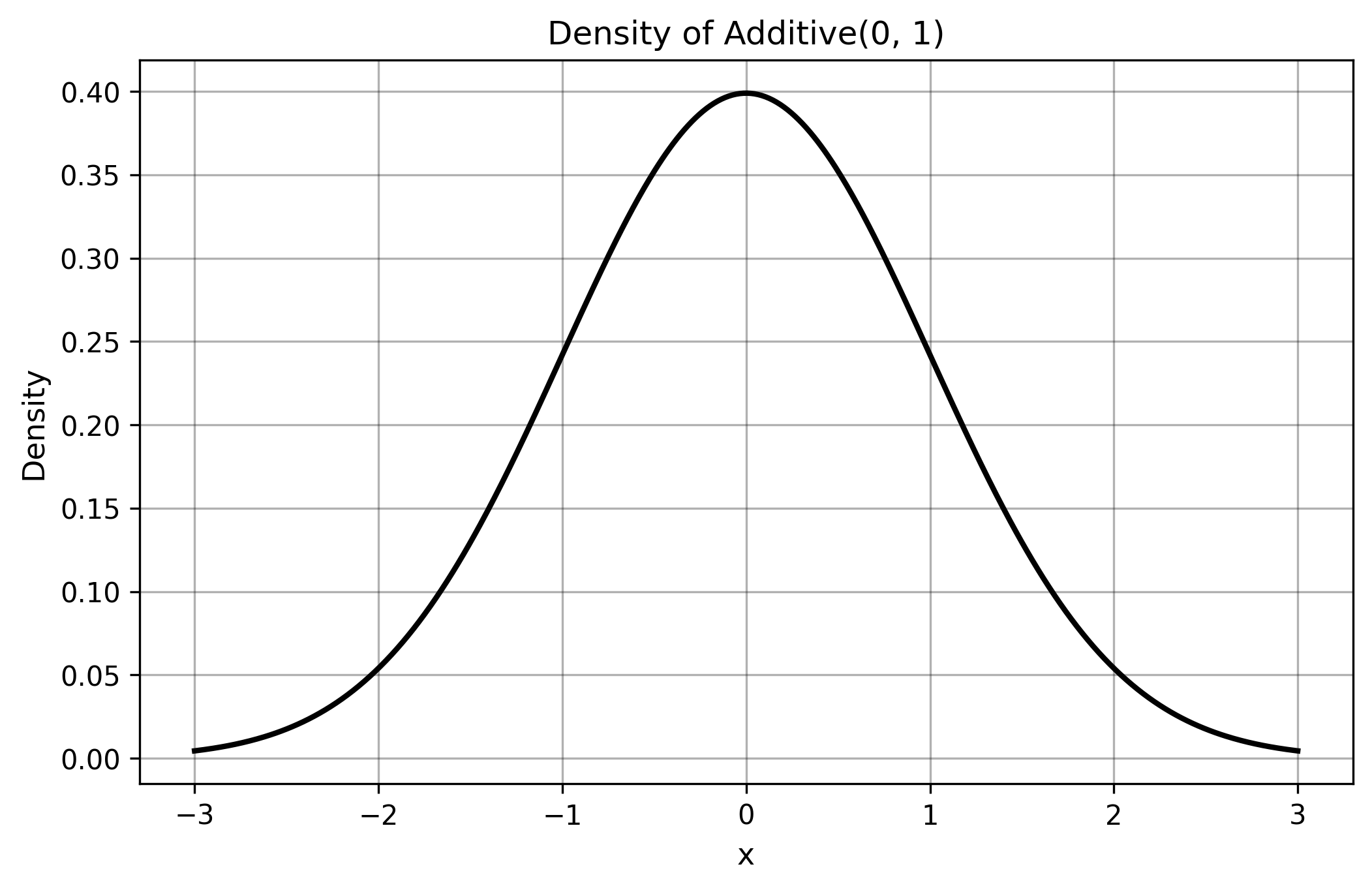
• Properties: symmetric, bell-shaped, characterized by central limit theorem convergence.
• Applications: measurement errors, heights and weights in populations, test scores, temperature variations.
• Characteristics: symmetric around the mean, light tails, finite variance.
• Caution: no perfectly additive distributions exist in real data; all real-world measurements contain deviations. Traditional estimators like $\operatorname{Mean}$ and $\operatorname{StdDev}$ lack robustness to outliers; use them only when strong evidence supports approximate additivity with no extreme measurements.

Notes

The $\underline{\operatorname{Additive}}$ (Normal) distribution has two parameters: the mean and the standard deviation, written as $\underline{\operatorname{Additive}}(\mathrm{mean}, \mathrm{stdDev})$.

Sampling (Box-Muller Transform)

The toolkit samples $\underline{\operatorname{Additive}}$ values using the Box-Muller transform (see Box & Muller 1958), which converts two independent $\operatorname{UniformFloat}$ draws into standard normal values. Given $U_1, U_2 in [0, 1)$:

Both $Z_0$ and $Z_1$ are independent standard normal values. The implementation uses only $Z_0$ to maintain cross-language determinism.

Asymptotic Spread Value

Consider two independent draws $X$ and $Y$ from the $\underline{\operatorname{Additive}}(\mathrm{mean}, \mathrm{stdDev})$ distribution. The goal is to find the median of their absolute difference $\lvert X-Y \rvert$. Define the difference $D = X - Y$. By linearity of expectation, $\mathbb{E}[D] = 0$. By independence, $\operatorname{Var}[D] = 2 \cdot \mathrm{stdDev}^2$. Thus $D$ has distribution $\underline{\operatorname{Additive}}(0, \sqrt{2} \cdot \mathrm{stdDev})$, and the problem reduces to finding the median of $\lvert D \rvert$. The location parameter $\mathrm{mean}$ disappears, as expected, because absolute differences are invariant to shifts.

Let $\tau=\sqrt{2} \cdot \mathrm{stdDev}$, so that $D \sim \underline{\operatorname{Additive}}(0, \tau)$. The random variable $\lvert D \rvert$ then follows the Half-$\underline{\operatorname{Additive}}$ (Folded Normal) distribution with scale $\tau$. Its cumulative distribution function for $z \geq 0$ becomes

where $\Phi$ denotes the standard $\underline{\operatorname{Additive}}$ (Normal) CDF.

The median $m$ is the point at which this cdf equals $\frac{1}{2}$. Setting $F_{\lvert D \rvert}(m)=\frac{1}{2}$ gives

Applying the inverse cdf yields $\frac{m}{\tau} = z_{0.75}$. Substituting back $\tau = \sqrt{2} \cdot \mathrm{stdDev}$ produces

Define $z_{0.75} := \Phi^{-1}(0.75) \approx 0.6744897502$. Numerically, the median absolute difference is approximately $\sqrt{2} \cdot z_{0.75} \cdot \mathrm{stdDev} \approx 0.9538725524 \cdot \mathrm{stdDev}$. This expression depends only on the scale parameter $\mathrm{stdDev}$, not on the mean, reflecting the translation invariance of the problem.

Lemma: Average Estimator Drift Formula

For average estimators $T_n$ with asymptotic standard deviation $a \cdot \frac{\mathrm{stdDev}}{\sqrt{n}}$ around the mean $\mu$, define $\operatorname{RelSpread}[T_n] := \frac{\operatorname{Spread}[T_n]}{\operatorname{Spread}[X]}$. In the $\underline{\operatorname{Additive}}$ (Normal) case, $\operatorname{Spread}[X] = \sqrt{2} \cdot z_{0.75} \cdot \mathrm{stdDev}$.

For any average estimator $T_n$ with asymptotic standard deviation $a \cdot \frac{\mathrm{stdDev}}{\sqrt{n}}$ around the mean $\mu$, the drift calculation follows:

• The spread of two independent estimates: $\operatorname{Spread}[T_n] = \sqrt{2} \cdot z_{0.75} \cdot a \cdot \frac{\mathrm{stdDev}}{\sqrt{n}}$
• The relative spread: $\operatorname{RelSpread}[T_n] = \frac{a}{\sqrt{n}}$
• The asymptotic drift: $\operatorname{Drift}(T, X) = a$

Asymptotic Mean Drift

For the sample mean $\operatorname{Mean}(\mathbf{x}) = \frac{1}{n} \sum_{i=1}^n x_i$ applied to samples from $\underline{\operatorname{Additive}}(\mathrm{mean}, \mathrm{stdDev})$, the sampling distribution of $\operatorname{Mean}$ is also additive with mean $\mathrm{mean}$ and standard deviation $\frac{\mathrm{stdDev}}{\sqrt{n}}$.

Using the lemma with $a = 1$ (since the standard deviation is $\frac{\mathrm{stdDev}}{\sqrt{n}}$):

$\operatorname{Mean}$ achieves unit drift under the $\underline{\operatorname{Additive}}$ (Normal) distribution, serving as the natural baseline for comparison. $\operatorname{Mean}$ is the optimal estimator under the $\underline{\operatorname{Additive}}$ (Normal) distribution: no other estimator achieves lower $\operatorname{Drift}$.

Asymptotic Median Drift

For the sample median $\operatorname{Median}(\mathbf{x})$ applied to samples from $\underline{\operatorname{Additive}}(\mathrm{mean}, \mathrm{stdDev})$, the asymptotic sampling distribution of $\operatorname{Median}$ is approximately $\underline{\operatorname{Additive}}$ (Normal) with mean $\mathrm{mean}$ and standard deviation $\sqrt{\frac{\pi}{2}} \cdot \frac{\mathrm{stdDev}}{\sqrt{n}}$.

This result follows from the asymptotic theory of order statistics. For the median of a sample from a continuous distribution with density $f$ and cumulative distribution $F$, the asymptotic variance is $\frac{1}{4n[f(F^{-1}(0.5))]^2}$. For the $\underline{\operatorname{Additive}}$ (Normal) distribution with standard deviation $\mathrm{stdDev}$, the density at the median (which equals the mean) is $\frac{1}{\mathrm{stdDev} \sqrt{2 \pi}}$. Thus the asymptotic variance becomes $\pi \cdot \mathrm{stdDev}^\frac{2}{2n}$.

Using the lemma with $a = \sqrt{\frac{\pi}{2}}$:

Numerically, $\sqrt{\frac{\pi}{2}} \approx 1.2533$, so the median has approximately 25% higher drift than the mean under the $\underline{\operatorname{Additive}}$ (Normal) distribution.

Asymptotic Center Drift

For the sample center $\operatorname{Center}(\mathbf{x}) = \underset{1 \leq i \leq j \leq n}{\operatorname{Median}} \frac{x_i + x_j}{2}$ applied to samples from $\underline{\operatorname{Additive}}(\mathrm{mean}, \mathrm{stdDev})$, its asymptotic sampling distribution must be determined.

The center estimator computes all pairwise averages (including $i=j$) and takes their median. For the $\underline{\operatorname{Additive}}$ (Normal) distribution, asymptotic theory shows that the center estimator is asymptotically $\underline{\operatorname{Additive}}$ (Normal) with mean $\mathrm{mean}$.

The exact asymptotic variance of the center estimator for the $\underline{\operatorname{Additive}}$ (Normal) distribution is:

This gives an asymptotic standard deviation of:

Using the lemma with $a = \sqrt{\frac{\pi}{3}}$:

Numerically, $\sqrt{\frac{\pi}{3}} \approx 1.0233$, so the center estimator achieves a drift very close to 1 under the $\underline{\operatorname{Additive}}$ (Normal) distribution, performing nearly as well as the mean while offering greater robustness to outliers.

Lemma: Dispersion Estimator Drift Formula

For dispersion estimators $T_n$ with asymptotic center $b \cdot \mathrm{stdDev}$ and standard deviation $a \cdot \frac{\mathrm{stdDev}}{\sqrt{n}}$, define $\operatorname{RelSpread}[T_n] := \frac{\operatorname{Spread}[T_n]}{b \cdot \mathrm{stdDev}}$.

For any dispersion estimator $T_n$ with asymptotic distribution $T_n \sim\text{approx} \underline{\operatorname{Additive}}(b \cdot \mathrm{stdDev}, (a \cdot \mathrm{stdDev})^\frac{2}{n})$, the drift calculation follows:

• The spread of two independent estimates: $\operatorname{Spread}[T_n] = \sqrt{2} \cdot z_{0.75} \cdot a \cdot \frac{\mathrm{stdDev}}{\sqrt{n}}$
• The relative spread: $\operatorname{RelSpread}[T_n] = \sqrt{2} \cdot z_{0.75} \cdot \frac{a}{b \sqrt{n}}$
• The asymptotic drift: $\operatorname{Drift}(T, X) = \sqrt{2} \cdot z_{0.75} \cdot \frac{a}{b}$

Note: The $\sqrt{2}$ factor comes from the standard deviation of the difference $D = T_1 - T_2$ of two independent estimates, and the $z_{0.75}$ factor converts this standard deviation to the median absolute difference.

Asymptotic StdDev Drift

For the sample standard deviation $\operatorname{StdDev}(\mathbf{x}) = \sqrt{\frac{1}{n-1} \sum_{i=1}^n (x_i - \operatorname{Mean}(\mathbf{x}))^2}$ applied to samples from $\underline{\operatorname{Additive}}(\mathrm{mean}, \mathrm{stdDev})$, the sampling distribution of $\operatorname{StdDev}$ is approximately $\underline{\operatorname{Additive}}$ (Normal) for large $n$ with mean $\mathrm{stdDev}$ and standard deviation $\frac{\mathrm{stdDev}}{\sqrt{2n}}$.

Applying the lemma with $a = \frac{1}{\sqrt{2}}$ and $b = 1$:

For the dispersion drift, we use the relative spread formula:

Since $\operatorname{Center}[\operatorname{StdDev}(X_{1:n})] \approx \mathrm{stdDev}$ asymptotically:

Therefore:

Numerically, $z_{0.75} \approx 0.67449$.

Asymptotic MAD Drift

For the median absolute deviation $\operatorname{MAD}(\mathbf{x}) = \operatorname{Median}(\lvert x_i - \operatorname{Median}(\mathbf{x}) \rvert)$ applied to samples from $\underline{\operatorname{Additive}}(\mathrm{mean}, \mathrm{stdDev})$, the asymptotic distribution is approximately $\underline{\operatorname{Additive}}$ (Normal).

For the $\underline{\operatorname{Additive}}$ (Normal) distribution, the population MAD equals $z_{0.75} \cdot \mathrm{stdDev}$. The asymptotic standard deviation of the sample MAD is:

where $c_{\mathrm{mad}} \approx 0.78$.

Applying the lemma with $a = c_{\mathrm{mad}}$ and $b = z_{0.75}$:

Since $\operatorname{Center}[\operatorname{MAD}(X_{1:n})] \approx z_{0.75} \cdot \mathrm{stdDev}$ asymptotically:

Therefore:

Numerically, $\sqrt{2} \cdot c_{\mathrm{mad}} \approx \sqrt{2} \cdot 0.78 \approx 1.10$.

Asymptotic Spread Drift

For the sample spread $\operatorname{Spread}(\mathbf{x}) = \underset{1 \leq i < j \leq n}{\operatorname{Median}} \lvert x_i - x_j \rvert$ applied to samples from $\underline{\operatorname{Additive}}(\mathrm{mean}, \mathrm{stdDev})$, the asymptotic distribution is approximately $\underline{\operatorname{Additive}}$ (Normal).

The spread estimator computes all pairwise absolute differences and takes their median. For the $\underline{\operatorname{Additive}}$ (Normal) distribution, the population spread equals $\sqrt{2} \cdot z_{0.75} \cdot \mathrm{stdDev}$ as derived in the Asymptotic Spread Value section.

The asymptotic standard deviation of the sample spread for the $\underline{\operatorname{Additive}}$ (Normal) distribution is:

where $c_{\mathrm{spr}} \approx 0.72$.

Applying the lemma with $a = c_{\mathrm{spr}}$ and $b = \sqrt{2} \cdot z_{0.75}$:

Since $\operatorname{Center}[\operatorname{Spread}(X_{1:n})] \approx \sqrt{2} \cdot z_{0.75} \cdot \mathrm{stdDev}$ asymptotically:

Therefore:

Numerically, $c_{\mathrm{spr}} \approx 0.72$.

Summary

Summary for average estimators:

The squared drift values indicate the sample size adjustment needed when switching estimators. For instance, switching from $\operatorname{Mean}$ to $\operatorname{Median}$ while maintaining the same precision requires increasing the sample size by a factor of $\frac{\pi}{2} \approx 1.571$ (about 57% more observations). Similarly, switching from $\operatorname{Mean}$ to $\operatorname{Center}$ requires only about 5% more observations.

The inverse squared drift (rightmost column) equals the classical statistical efficiency relative to the $\operatorname{Mean}$. The $\operatorname{Mean}$ achieves optimal performance (unit efficiency) for the $\underline{\operatorname{Additive}}$ (Normal) distribution, as expected from classical theory. The $\operatorname{Center}$ maintains 95.5% efficiency while offering greater robustness to outliers, making it an attractive alternative when some contamination is possible. The $\operatorname{Median}$, while most robust, operates at only 63.7% efficiency under purely $\underline{\operatorname{Additive}}$ (Normal) conditions.

Summary for dispersion estimators:

For the $\underline{\operatorname{Additive}}$ (Normal) distribution, the asymptotic drift values reveal the relative precision of different dispersion estimators:

The squared drift values indicate the sample size adjustment needed when switching estimators. For instance, switching from $\operatorname{StdDev}$ to $\operatorname{MAD}$ while maintaining the same precision requires increasing the sample size by a factor of $1.\frac{22}{0}.45 \approx 2.71$ (more than doubling the observations). Similarly, switching from $\operatorname{StdDev}$ to $\operatorname{Spread}$ requires a factor of $0.\frac{52}{0}.45 \approx 1.16$.

The $\operatorname{StdDev}$ achieves optimal performance for the $\underline{\operatorname{Additive}}$ (Normal) distribution. The $\operatorname{MAD}$ requires about 2.7 times more data to match the $\operatorname{StdDev}$ precision while offering greater robustness to outliers. The $\operatorname{Spread}$ requires about 1.16 times more data to match the $\operatorname{StdDev}$ precision under purely $\underline{\operatorname{Additive}}$ (Normal) conditions while maintaining robustness.