Pragmastat: Pragmatic Statistical Toolkit
Pragmastat:
Pragmatic Statistical Toolkit
DOI: 10.5281/zenodo.17236778
This manual presents a toolkit of statistical procedures that provide reliable results across diverse real-world distributions, with ready-to-use implementations and detailed explanations. The toolkit consists of renamed, recombined, and refined versions of existing methods. Written for software developers, mathematicians, and LLMs.
▼
Table of Content
§1. Introduction
§1.1. Primer
Given two numeric samples $\x = (x_1, \ldots, x_n)$ and $\y = (y_1, \ldots, y_m)$, the toolkit provides the following primary procedures:
$\Center(\x) = \underset{1 \leq i \leq j \leq n}{\Median} \left((x_i + x_j)/2 \right)$ — robust average of $\x$
For $\x = (0, 2, 4, 6, 8)$:
$$ \begin{aligned} \Center(\x) &= 4 \\ \Center(\x + 10) &= 14 \\ \Center(3\x) &= 12 \end{aligned} $$$\Spread(\x) = \underset{1 \leq i < j \leq n}{\Median} |x_i - x_j|$ — robust dispersion of $\x$
For $\x = (0, 2, 4, 6, 8)$:
$$ \begin{aligned} \Spread(\x) &= 4 \\ \Spread(\x + 10) &= 4 \\ \Spread(2\x) &= 8 \end{aligned} $$$\RelSpread(\x) = \Spread(\x) / \left| \Center(\x) \right|$ — robust relative dispersion of $\x$
For $\x = (0, 2, 4, 6, 8)$:
$$ \begin{aligned} \RelSpread(\x) &= 1 \\ \RelSpread(5\x) &= 1 \end{aligned} $$$\Shift(\x, \y) = \underset{1 \leq i \leq n, 1 \leq j \leq m}{\Median} \left(x_i - y_j \right)$ — robust signed difference ($\x-\y$)
For $\x = (0, 2, 4, 6, 8)$ and $\y = (10, 12, 14, 16, 18)$:
$$ \begin{aligned} \Shift(\x, \y) &= -10 \\ \Shift(\x, \x) &= 0 \\ \Shift(\x + 7, \y + 3) &= -6 \\ \Shift(2\x, 2\y) &= -20 \\ \Shift(\y, \x) &= 10 \end{aligned} $$$\Ratio(\x, \y) = \underset{1 \leq i \leq n, 1 \leq j \leq m}{\Median} \left( x_i / y_j \right)$ — robust ratio ($\x/\y$)
For $\x = (1, 2, 4, 8, 16)$ and $\y = (2, 4, 8, 16, 32)$:
$$ \begin{aligned} \Ratio(\x, \y) &= 0.5 \\ \Ratio(\x, \x) &= 1 \\ \Ratio(2\x, 5\y) &= 0.2 \end{aligned} $$$\AvgSpread(\x, \y) = (n\Spread(\x) + m\Spread(\y)) / (n + m)$ — robust average spread of $\x$ and $\y$
For $\x = (0, 3, 6, 9, 12)$ and $\y = (0, 2, 4, 6, 8)$:
$$ \begin{aligned} \Spread(\x) &= 6 \\ \Spread(\y) &= 4 \\ \AvgSpread(\x, \y) &= 5 \\ \AvgSpread(\x, \x) &= 6 \\ \AvgSpread(2\x, 3\x) &= 15 \\ \AvgSpread(\y, \x) &= 5 \\ \AvgSpread(2\x, 2\y) &= 10 \end{aligned} $$$\Disparity(\x, \y) = \Shift(\x, \y) / \AvgSpread(\x, \y)$ — robust effect size between $\x$ and $\y$
For $\x = (0, 3, 6, 9, 12)$ and $\y = (0, 2, 4, 6, 8)$:
$$ \begin{aligned} \Shift(\x, \y) &= 2 \\ \AvgSpread(\x, \y) &= 5 \\ \Disparity(\x, \y) &= 0.4 \\ \Disparity(\x + 5, \y + 5) &= 0.4 \\ \Disparity(2\x, 2\y) &= 0.4 \\ \Disparity(\y, \x) &= -0.4 \end{aligned} $$These procedures are designed to serve as default choices for routine analysis and comparison tasks in engineering contexts. The toolkit has ready-to-use implementations for Python, TypeScript/JavaScript, R, C#, Kotlin, Rust, and Go.
§1.2. Breaking changes
Statistical practice has evolved through decades of research and teaching, creating a system where historical naming conventions became embedded in textbooks and standard practice. Traditional statistics often names procedures after their discoverers or uses arbitrary symbols that reveal nothing about their actual purpose or application context. This approach forces practitioners to memorize meaningless mappings between historical figures and mathematical concepts.
The result is unnecessary friction for anyone learning or applying statistical methods. Beginners face an inconsistent landscape of confusing names, fragile defaults, and incompatible approaches with little guidance on selection or interpretation. Modern practitioners would benefit from a more consistent system, which requires some renaming and redefining. This manual offers a coherent system designed for clarity and practical use, breaking from tradition. The following concepts were adopted from traditional textbooks via renaming or reworking:
- Estimators
- Average: $\Center$ (former ‘Hodges-Lehmann location estimator’)
- Dispersion: $\Spread$ (former ‘Shamos scale estimator’)
- Effect Size: $\Disparity$ (a robust alternative to ‘Cohen’s $d$’)
- Estimator properties
- Precision: $\Drift$ (a robust alternative to statistical efficiency)
- Distributions
- $\Additive$ (former ‘Normal’ or ‘Gaussian’)
- $\Multiplic$ (former ‘Log-Normal’ or ‘Galton’)
- $\Power$ (former ‘Pareto’)
§1.3. Definitions
- $X$, $Y$: random variables, can be treated as generators of random real measurements
- $X \sim \underline{\operatorname{Distribution}}$ defines a distribution from which this variable comes
- $x_i, y_j$: specific individual measurements
- $\x = (x_1, x_2, \ldots, x_n)$, $\y = (y_1, y_2, \ldots, y_m)$: samples of measurements of a given size
- Samples are non-empty: $n, m \geq 1$
- $x_{(1)}, x_{(2)}, \ldots, x_{(n)}$: sorted measurements of the sample (‘order statistics’)
- Asymptotic case: the sample size goes to infinity $n, m \to \infty$
- Can typically be treated as an approximation for large samples
- $\operatorname{Estimator}(\x)$: a function that estimates the property of a distribution from given measurements
- $\operatorname{Estimator}[X]$ shows the true property value of the distribution (asymptotic value)
- $\Median$: an estimator that finds the value splitting the distribution into two equal parts
§2. Summary Estimators
The following sections introduce definitions of one-sample and two-sample summary estimators. Later sections will evaluate properties of these estimators and applicability to different conditions.
§2.1. Center
$$ \Center(\x) = \underset{1 \leq i \leq j \leq n}{\Median} \left(\frac{x_i + x_j}{2} \right) $$- Measures average (central tendency, measure of location)
- Equals the Hodges-Lehmann estimator (hodges1963, sen1963), renamed to $\Center$ for clarity
- Also known as ‘pseudomedian’ because it is consistent with $\Median$ for symmetric distributions
- Pragmatic alternative to $\Mean$ and $\Median$
- Asymptotically, $\Center[X]$ is the $\Median$ of the arithmetic average of two random measurements from $X$
- Straightforward implementations have $O(n^2 \log n)$ complexity; a fast $O(n \log n)$ version is provided in the Algorithms section.
- Domain: any real numbers
- Unit: the same as measurements
§2.2. Spread
$$ \Spread(\x) = \underset{1 \leq i < j \leq n}{\Median} |x_i - x_j| $$- Measures dispersion (variability, scatter)
- Corner case: for $n=1$, $\Spread(\x) = 0$
- Equals the Shamos scale estimator (shamos1976), renamed to $\Spread$ for clarity
- Pragmatic alternative to the standard deviation and the median absolute deviation
- Asymptotically, $\Spread[X]$ is the median of the absolute difference between two random measurements from distribution $X$
- Straightforward implementations have $O(n^2 \log n)$ complexity; a fast $O(n \log n)$ version is provided in the Algorithms section.
- Domain: any real numbers
- Unit: the same as measurements
§2.3. RelSpread
$$ \RelSpread(\x) = \frac{\Spread(\x)}{\left| \Center(\x) \right|} $$- Measures the relative dispersion of a sample to $\Center(\x)$
- Pragmatic alternative to the coefficient of variation
- Domain: $\Center(\x) \neq 0$
- Unit: relative
§2.4. Shift
$$ \Shift(\x, \y) = \underset{1 \leq i \leq n,\,\, 1 \leq j \leq m}{\Median} \left(x_i - y_j \right) $$- Measures the median of pairwise differences between elements of two samples
- Equals the Hodges-Lehmann estimator for two samples (hodges1963)
- Asymptotically, $\Shift[X, Y]$ is the median of the difference of random measurements from $X$ and $Y$
- Straightforward implementations have $O(mn \log(mn))$ complexity; a fast $O((m+n) \log L)$ version is provided in the Algorithms section.
- Domain: any real numbers
- Unit: the same as measurements
§2.5. Ratio
$$ \Ratio(\x, \y) = \underset{1 \leq i \leq n, 1 \leq j \leq m}{\Median} \left( \dfrac{x_i}{y_j} \right) $$- Measures the median of pairwise ratios between elements of two samples
- Asymptotically, $\Ratio[X, Y]$ is the median of the ratio of random measurements from $X$ and $Y$
- Note: $\Ratio(\x, \y) \neq 1 / \Ratio(\y, \x)$ in general (example: $x=(1, 100)$, $y=(1, 10)$)
- Practical Domain: $x_i, y_j > 0$ or $x_i, y_j < 0$. In practice, exclude values with $|y_j|$ near zero.
- Unit: relative
§2.6. AvgSpread
$$ \AvgSpread(\x, \y) = \dfrac{n\Spread(\x) + m\Spread(\y)}{n + m} $$- Measures average dispersion across two samples
- Pragmatic alternative to the ‘pooled standard deviation’
- Note: $\AvgSpread(\x, \y) \neq \Spread(\x \cup \y)$ in general (defines a pooled scale, not the spread of the concatenated sample)
- Domain: any real numbers
- Unit: the same as measurements
§2.7. Disparity (‘robust effect size’)
$$ \Disparity(\x, \y) = \dfrac{\Shift(\x, \y)}{\AvgSpread(\x, \y)} $$- Measures a normalized $\Shift$ between $\x$ and $\y$ expressed in spread units
- Expresses the ’effect size’, renamed to $\Disparity$ for clarity
- Pragmatic alternative to Cohen’s d (note: exact estimates differ due to robust construction)
- Domain: $\AvgSpread(\x, \y) > 0$
- Unit: spread unit
§3. Distributions
This section defines the distributions used throughout the manual.
§3.1. Additive (‘Normal’)
$$ \Additive(\mathrm{mean}, \mathrm{stdDev}) $$- $\mathrm{mean}$: location parameter (center of the distribution), consistent with $\Center$
- $\mathrm{stdDev}$: scale parameter (standard deviation), can be rescaled to $\Spread$
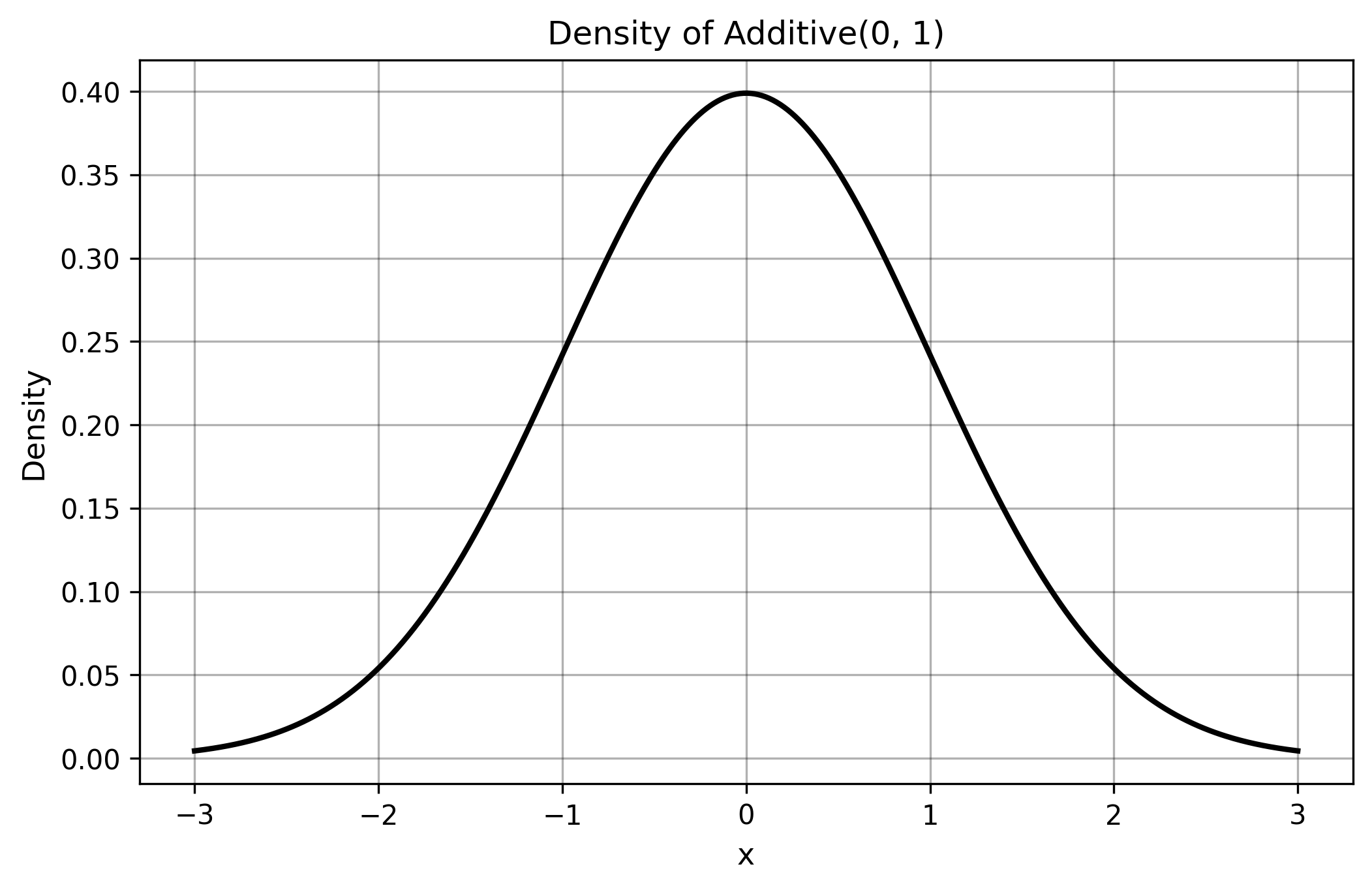
- Formation: the sum of many variables $X_1 + X_2 + \ldots + X_n$ under mild CLT (Central Limit Theorem) conditions (e.g., Lindeberg-Feller).
- Origin: historically called ‘Normal’ or ‘Gaussian’ distribution after Carl Friedrich Gauss and others.
- Rename Motivation: renamed to $\Additive$ to reflect its formation mechanism through addition.
- Properties: symmetric, bell-shaped, characterized by central limit theorem convergence.
- Applications: measurement errors, heights and weights in populations, test scores, temperature variations.
- Characteristics: symmetric around the mean, light tails, finite variance.
- Caution: no perfectly additive distributions exist in real data; all real-world measurements contain some deviations. Traditional estimators like $\Mean$ and $\StdDev$ lack robustness to outliers; use them only when strong evidence supports small deviations from additivity with no extreme measurements.
§3.2. Multiplic (‘LogNormal’)
$$ \Multiplic(\mathrm{logMean}, \mathrm{logStdDev}) $$- $\mathrm{logMean}$: mean of log values (location parameter; $e^{\mathrm{logMean}}$ equals the geometric mean)
- $\mathrm{logStdDev}$: standard deviation of log values (scale parameter; controls multiplicative spread)
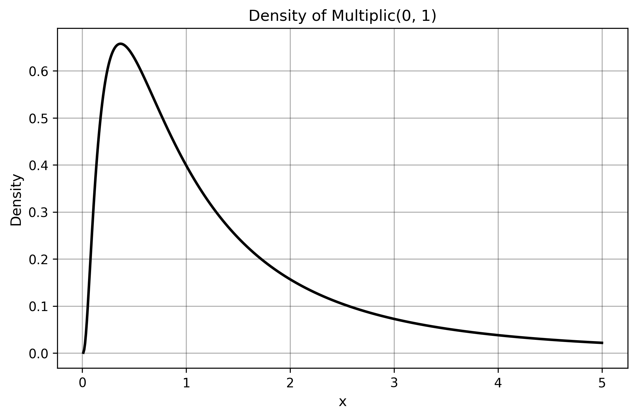
- Formation: the product of many positive variables $X_1 \cdot X_2 \cdot \ldots \cdot X_n$ with mild conditions (e.g., finite variance of $\log X$).
- Origin: historically called ‘Log-Normal’ or ‘Galton’ distribution after Francis Galton.
- Rename Motivation: renamed to $\Multiplic$ to reflect its formation mechanism through multiplication.
- Properties: logarithm of a $\Multiplic$ (‘LogNormal’) variable follows an $\Additive$ (‘Normal’) distribution.
- Applications: stock prices, file sizes, reaction times, income distributions, biological growth rates.
- Caution: no perfectly multiplic distributions exist in real data; all real-world measurements contain some deviations. Traditional estimators may struggle with the inherent skewness and heavy right tail.
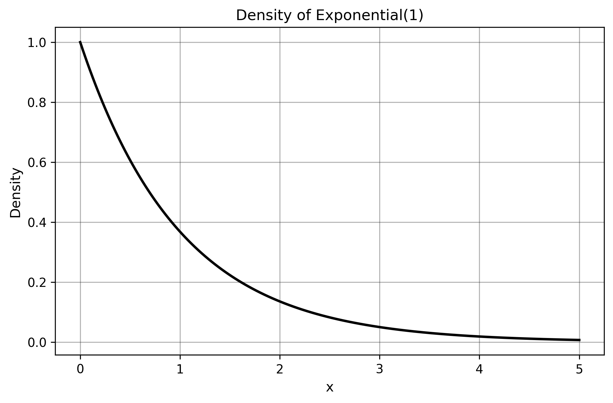
§3.3. Exponential
$$ \Exp(\mathrm{rate}) $$- $\mathrm{rate}$: rate parameter ($\lambda > 0$, controls decay speed; mean = $1/\mathrm{rate}$)
- Formation: the waiting time between events in a Poisson process.
- Origin: naturally arises from memoryless processes where the probability of an event occurring is constant over time.
- Properties: memoryless (past events do not affect future probabilities).
- Applications: time between failures, waiting times in queues, radioactive decay, customer service times.
- Characteristics: always positive, right-skewed with a light (exponential) tail.
- Caution: extreme skewness makes traditional location estimators like $\Mean$ unreliable; robust estimators provide more stable results.
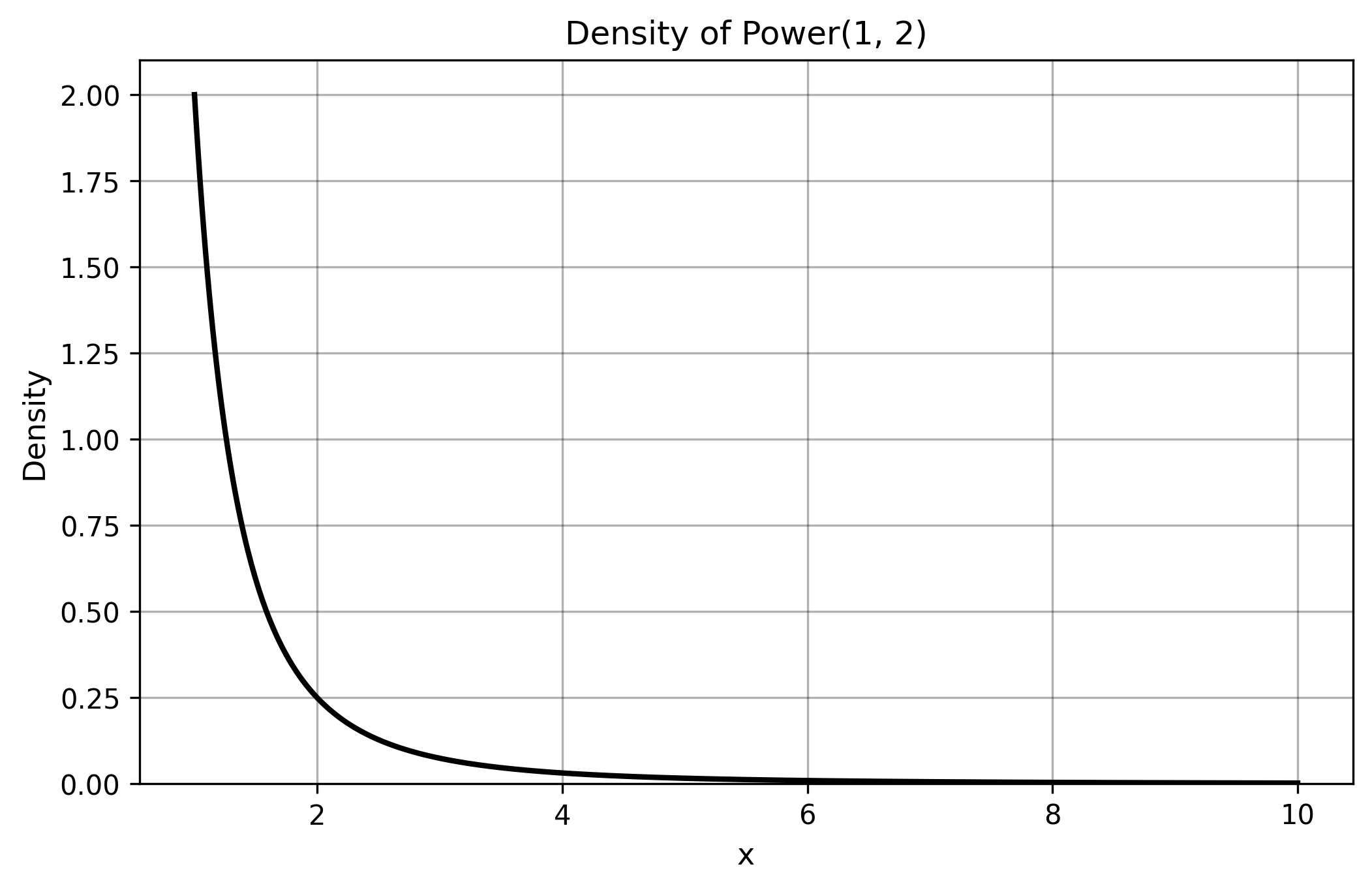
§3.4. Power (‘Pareto’)
$$ \Power(\mathrm{min}, \mathrm{shape}) $$- $\mathrm{min}$: minimum value (lower bound, $\mathrm{min} > 0$)
- $\mathrm{shape}$: shape parameter ($\alpha > 0$, controls tail heaviness; smaller values = heavier tails)
- Formation: follows a power-law relationship where large values are rare but possible.
- Origin: historically called ‘Pareto’ distribution after Vilfredo Pareto’s work on wealth distribution.
- Rename Motivation: renamed to $\Power$ to reflect its connection with power-law.
- Properties: exhibits scale invariance and extremely heavy tails.
- Applications: wealth distribution, city population sizes, word frequencies, earthquake magnitudes, website traffic.
- Characteristics: infinite variance for many parameter values; extreme outliers are common.
- Caution: traditional variance-based estimators completely fail; robust estimators are essential for reliable analysis.
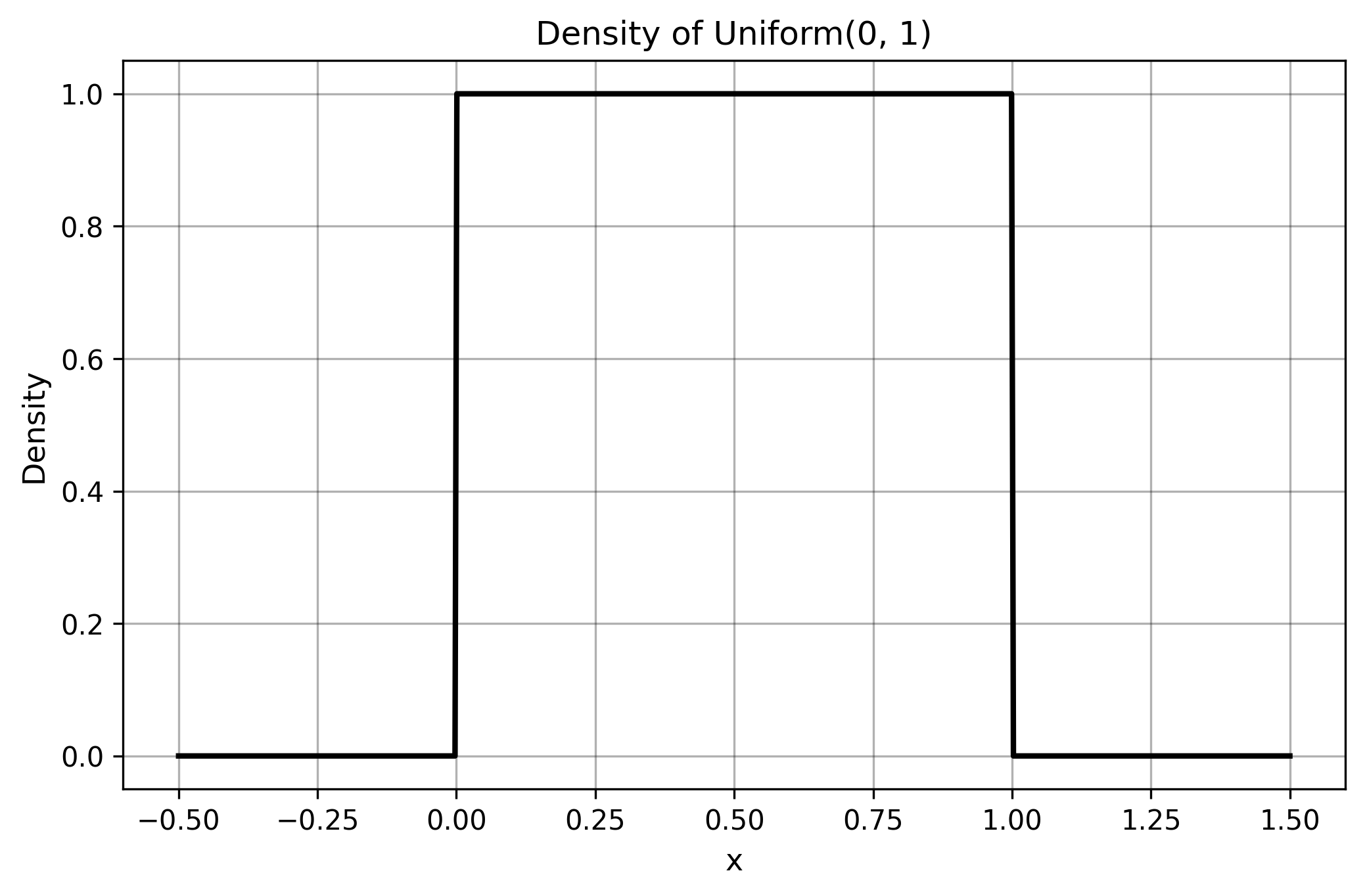
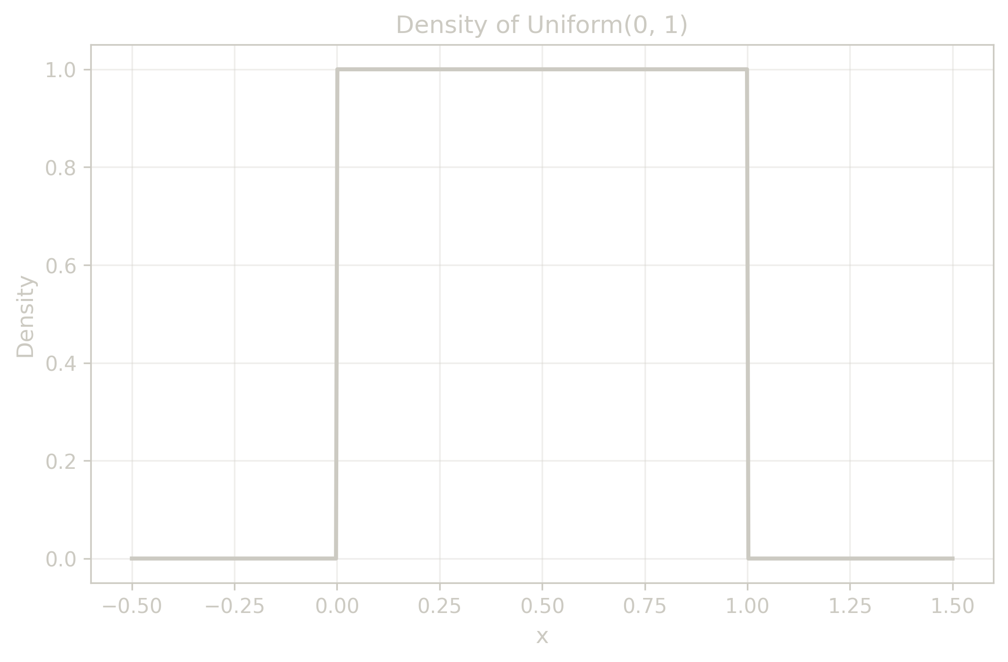
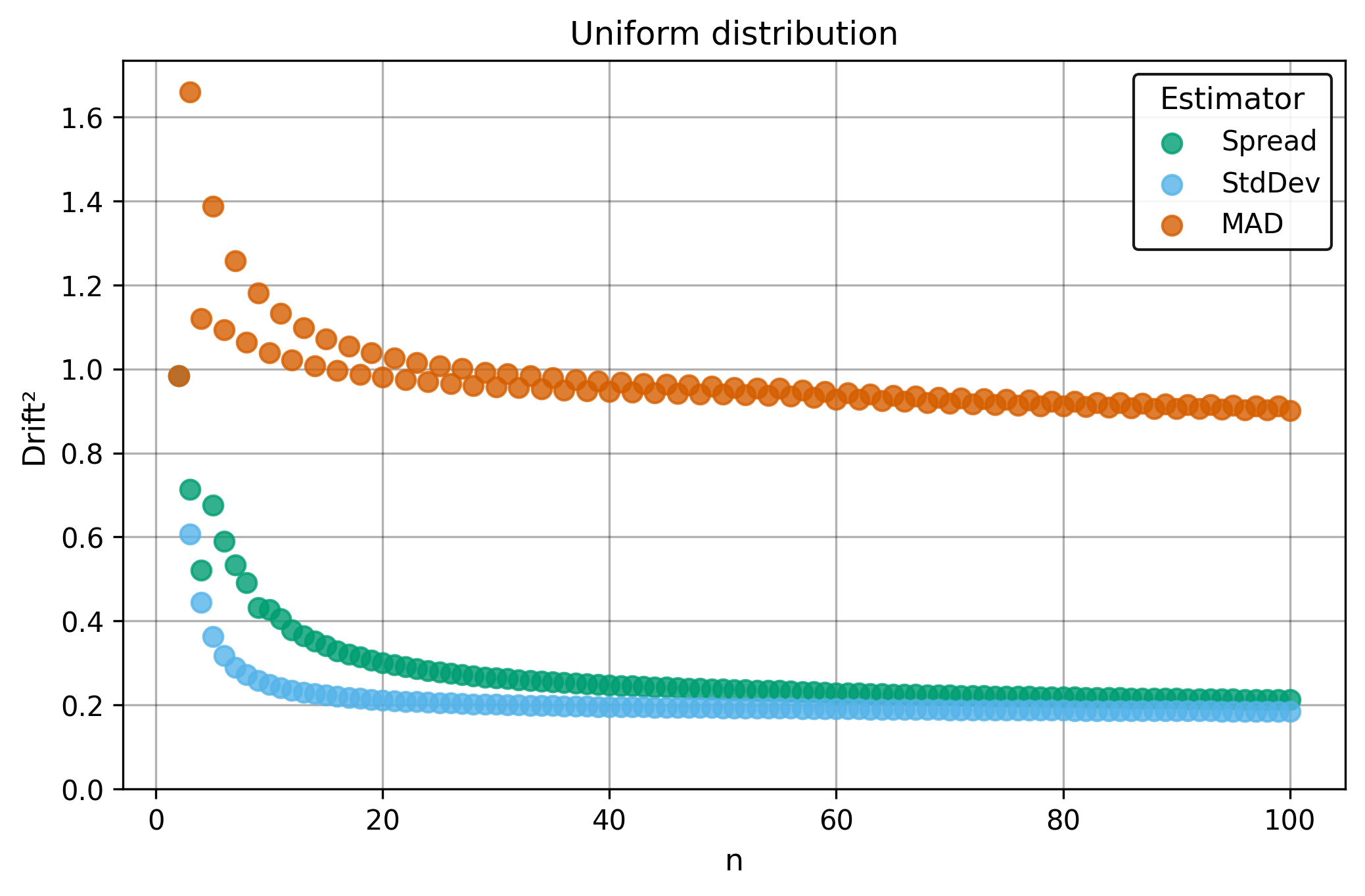
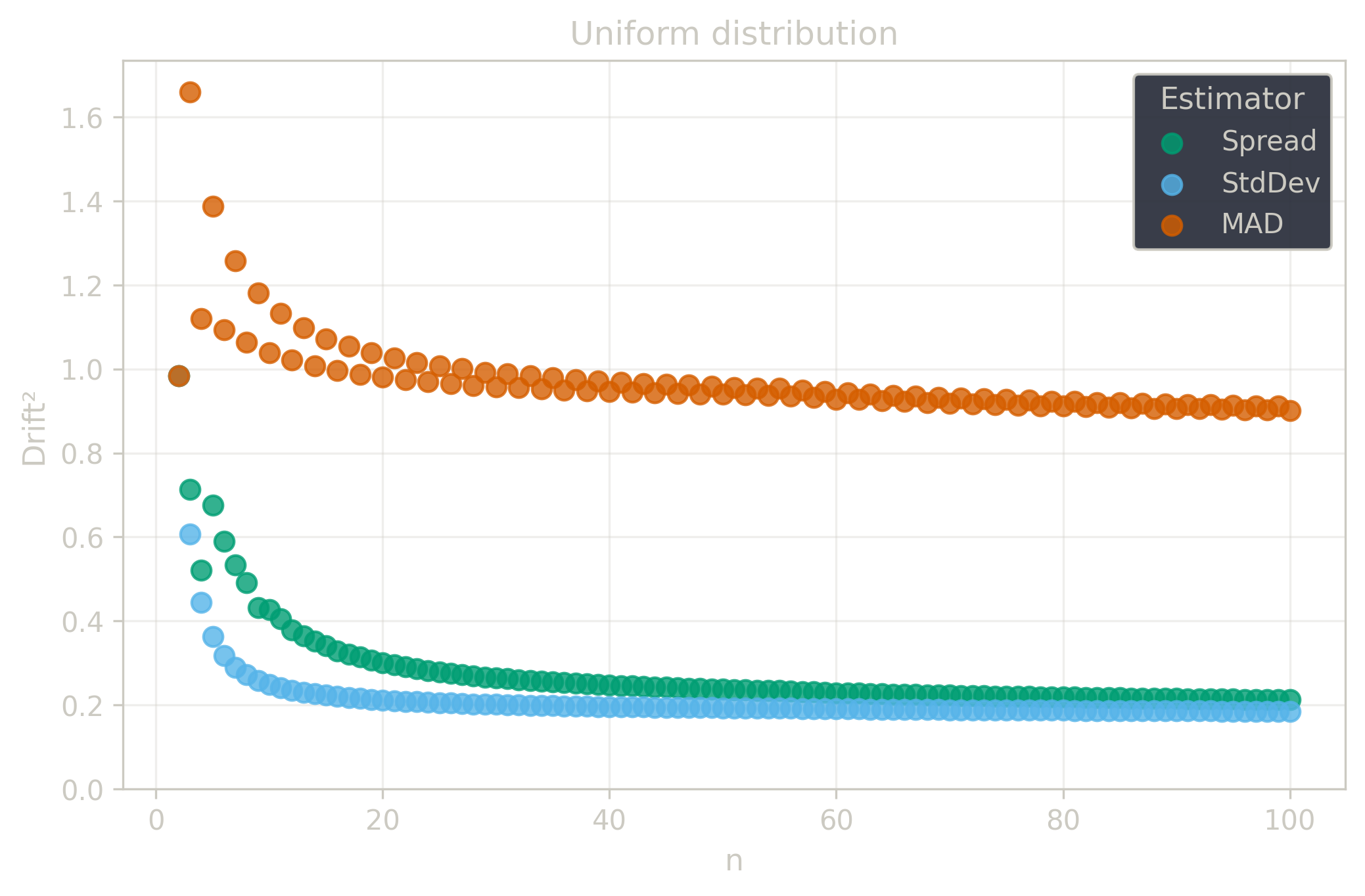
§3.5. Uniform
$$ \Uniform(\mathrm{min}, \mathrm{max}) $$- $\mathrm{min}$: lower bound of the support interval
- $\mathrm{max}$: upper bound of the support interval ($\mathrm{max} > \mathrm{min}$)
- Formation: all values within a bounded interval have equal probability.
- Origin: represents complete uncertainty within known bounds.
- Properties: rectangular probability density, finite support with hard boundaries.
- Applications: random number generation, round-off errors, arrival times within known intervals.
- Characteristics: symmetric, bounded, no tail behavior.
- Note: traditional estimators work reasonably well due to symmetry and bounded nature.
§4. Summary Estimator Properties
This section compares the toolkit’s robust estimators against traditional statistical methods to demonstrate their advantages and universally good properties. While traditional estimators often work well under ideal conditions, the toolkit’s estimators maintain reliable performance across diverse real-world scenarios.
Average Estimators:
Mean (arithmetic average):
$$ \Mean(\x) = \frac{1}{n} \sum_{i=1}^{n} x_i $$Median:
$$ \Median(\x) = \begin{cases} x_{((n+1)/2)} & \text{if } n \text{ is odd} \\ \frac{x_{(n/2)} + x_{(n/2+1)}}{2} & \text{if } n \text{ is even} \end{cases} $$Center (Hodges-Lehmann estimator):
$$ \Center(\x) = \underset{1 \leq i \leq j \leq n}{\Median} \left(\frac{x_i + x_j}{2} \right) $$Dispersion Estimators:
Standard Deviation:
$$ \StdDev(\x) = \sqrt{\frac{1}{n-1} \sum_{i=1}^{n} (x_i - \Mean(\x))^2} $$Median Absolute Deviation (around the median):
$$ \MAD(\x) = \Median(|x_i - \Median(\x)|) $$Spread (Shamos scale estimator):
$$ \Spread(\x) = \underset{1 \leq i < j \leq n}{\Median} |x_i - x_j| $$§4.1. Breakdown
Heavy-tailed distributions naturally produce extreme outliers that completely distort traditional estimators. A single extreme measurement from the $\Power$ distribution can make the sample mean arbitrarily large. Real-world data can also contain corrupted measurements from instrument failures, recording errors, or transmission problems. Both natural extremes and data corruption create the same challenge: extracting reliable information when some measurements are too influential.
The breakdown point is the fraction of a sample that can be replaced by arbitrarily large values without making an estimator arbitrarily large. The theoretical maximum is $50\%$; no estimator can guarantee reliable results when more than half the measurements are extreme or corrupted. In such cases, summary estimators are not applicable, and a more sophisticated approach is needed.
A $50\%$ breakdown point is rarely needed in practice, as more conservative values also cover practical needs. Additionally, a high breakdown point corresponds to low precision (information is lost by neglecting part of the data). The optimal practical breakdown point should be between $0\%$ (no robustness) and $50\%$ (low precision).
The $\Center$ and $\Spread$ estimators achieve $29\%$ breakdown points, providing substantial protection against realistic contamination levels while maintaining good precision. Below is a comparison with traditional estimators.
Asymptotic breakdown points for average estimators:
| $\Mean$ | $\Median$ | $\Center$ |
|---|---|---|
| 0% | 50% | 29% |
Asymptotic breakdown points for dispersion estimators:
| $\StdDev$ | $\MAD$ | $\Spread$ |
|---|---|---|
| 0% | 50% | 29% |
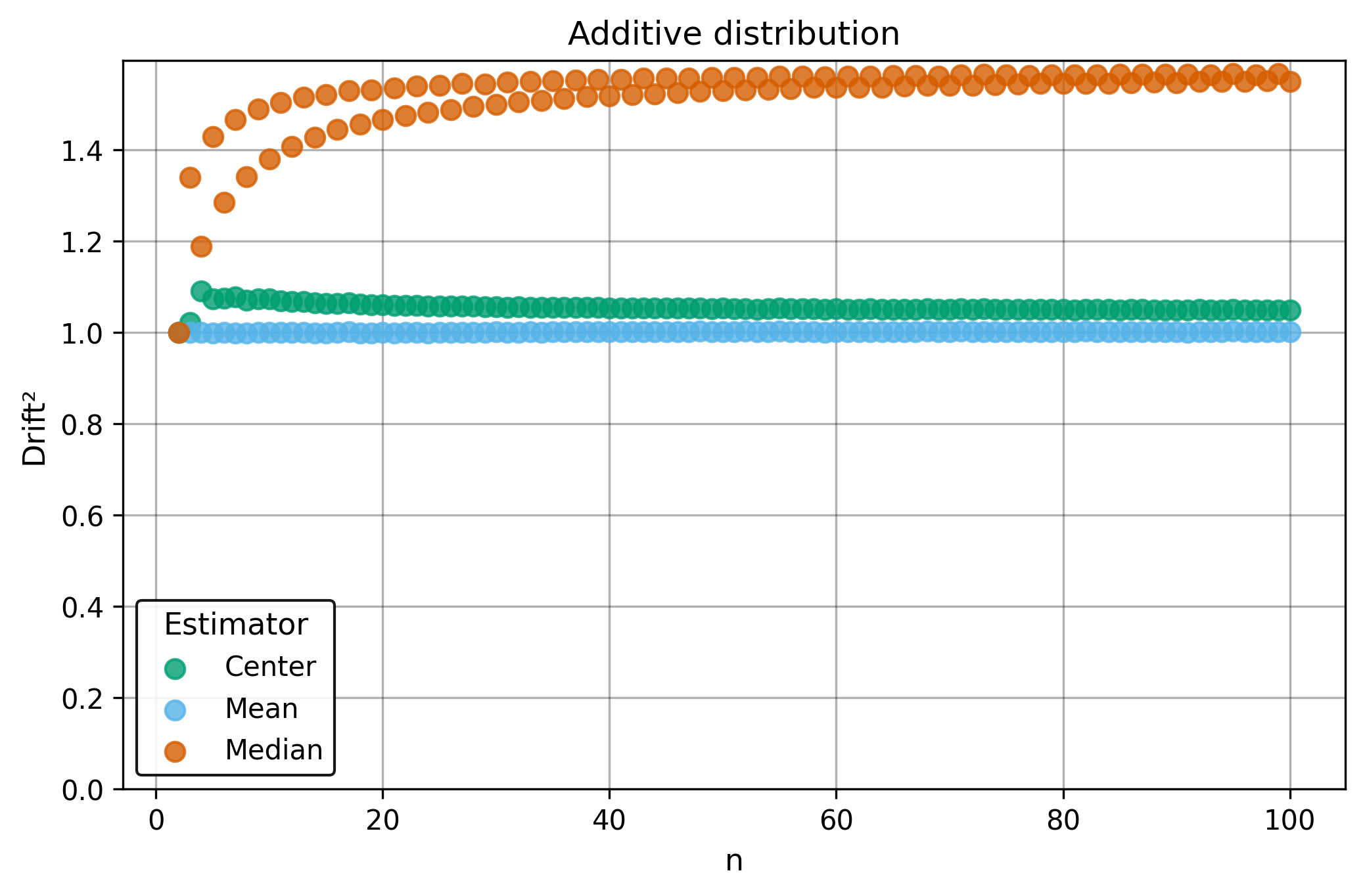
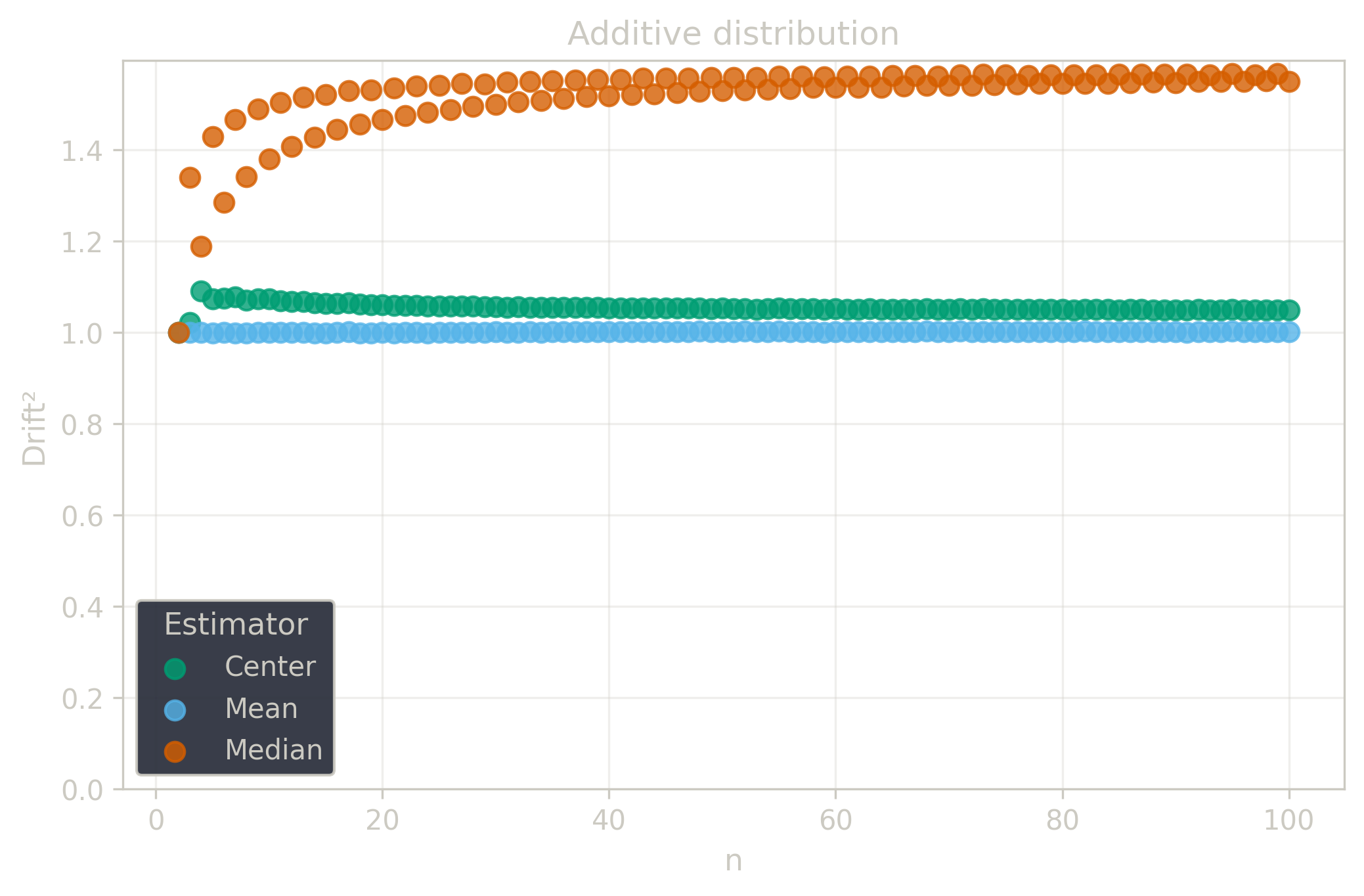
§4.2. Drift
Drift measures estimator precision by quantifying how much estimates scatter across repeated samples. It is based on the $\Spread$ of estimates and therefore has a breakdown point of approximately $29\%$.
Drift is useful for comparing the precision of several estimators. To simplify the comparison, one of the estimators can be chosen as a baseline. A table of squared drift values, normalized by the baseline, shows the required sample size adjustment factor for switching from the baseline to another estimator. For example, if $\Center$ is the baseline and the rescaled drift square of $\Median$ is $1.5$, this means that $\Median$ requires $1.5$ times more data than $\Center$ to achieve the same precision. See the “From Statistical Efficiency to Drift” section for details.
Squared Asymptotic Drift of Average Estimators (values are approximated):
| $\Mean$ | $\Median$ | $\Center$ | |
|---|---|---|---|
| $\Additive$ | 1.0 | 1.571 | 1.047 |
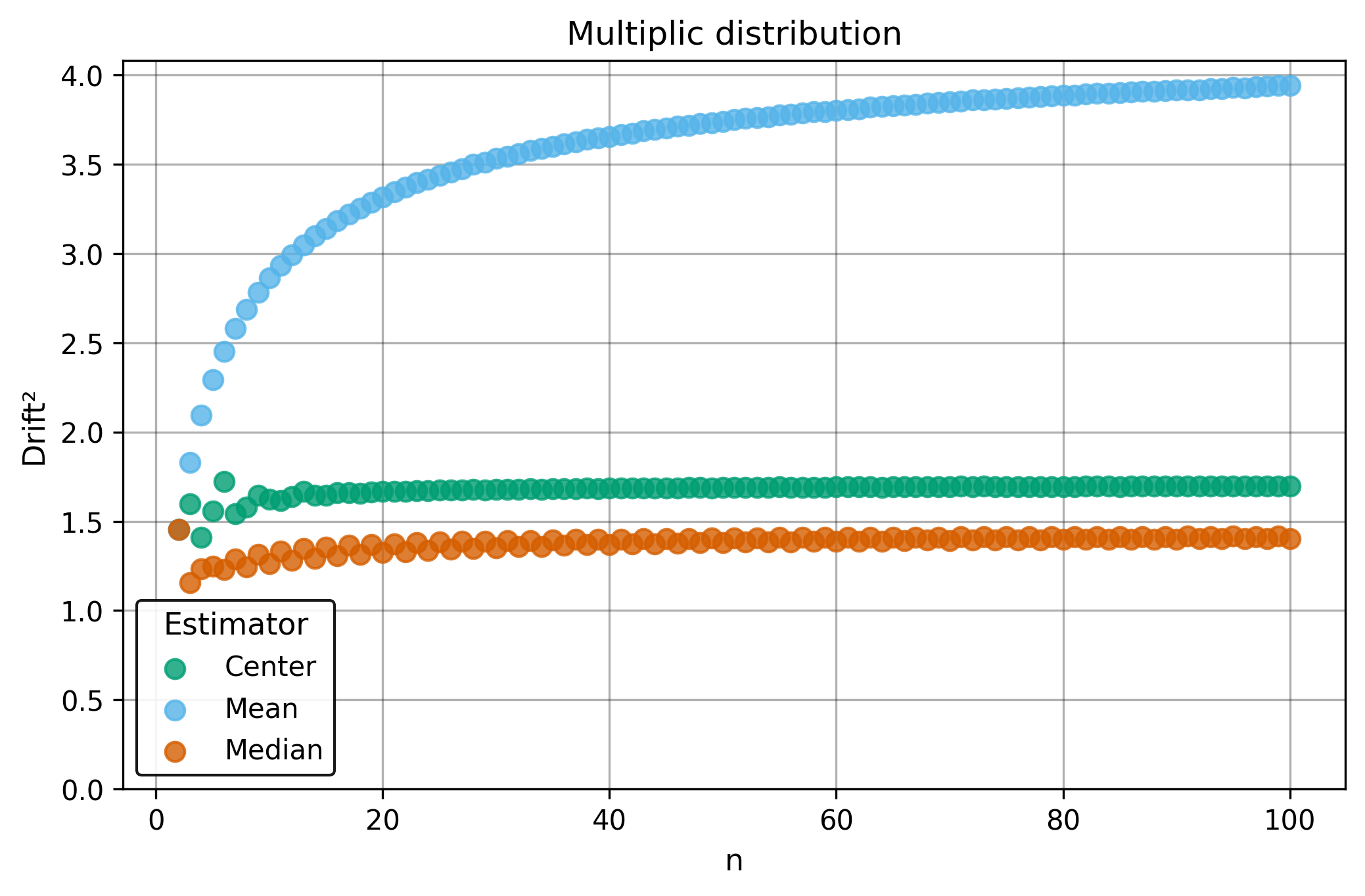
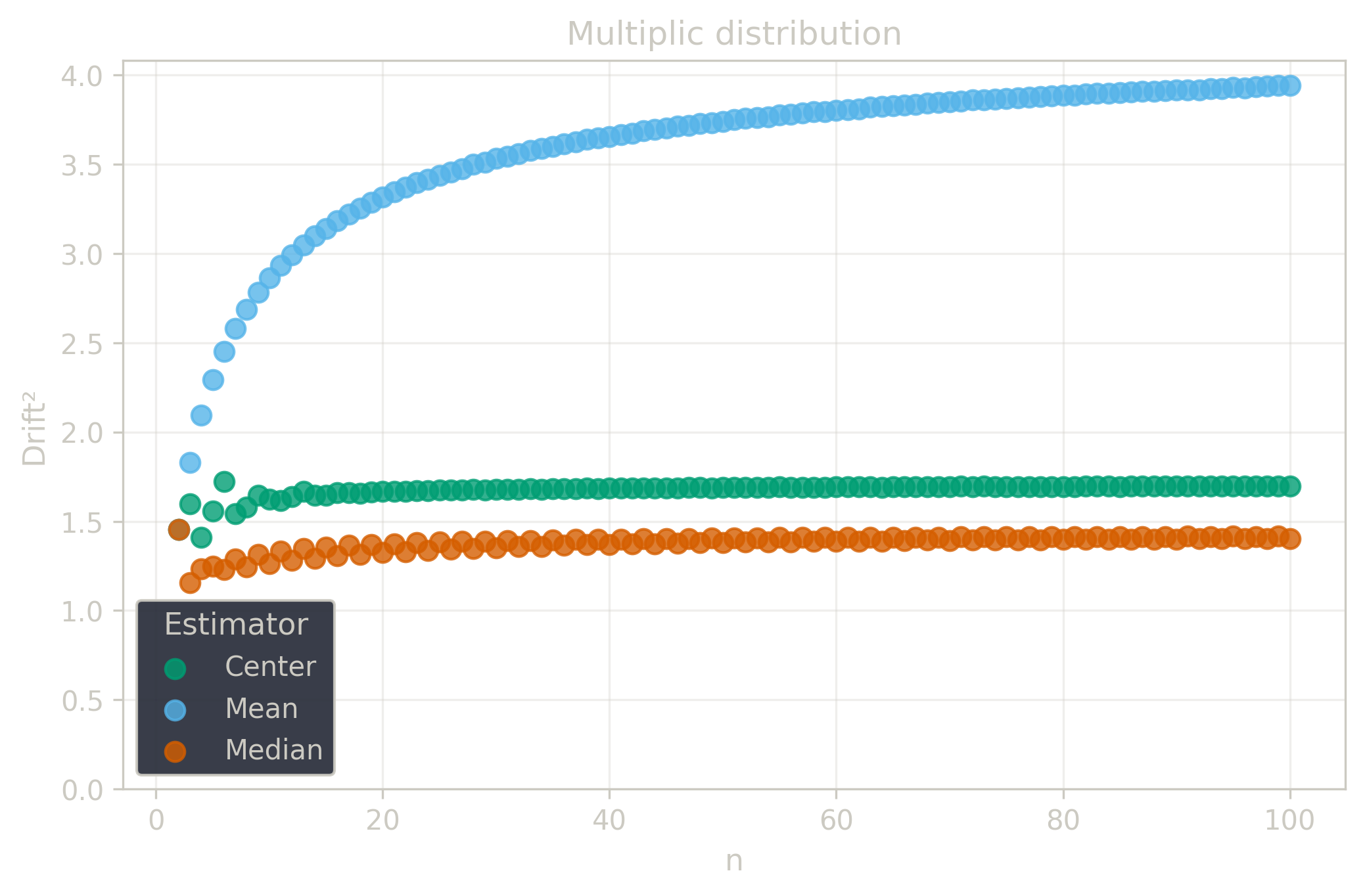
| $\Multiplic$ | 3.95 | 1.40 | 1.7 |
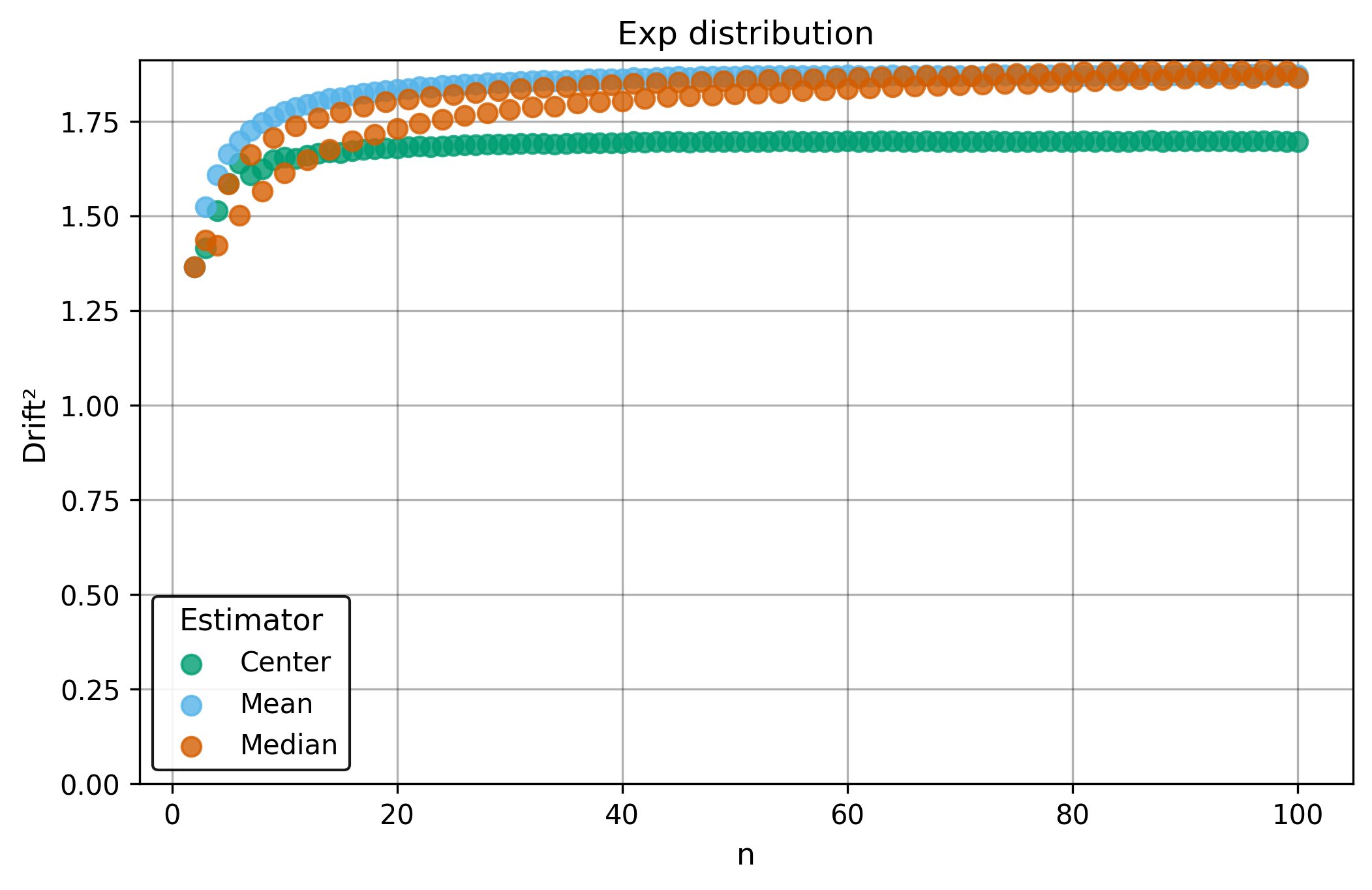
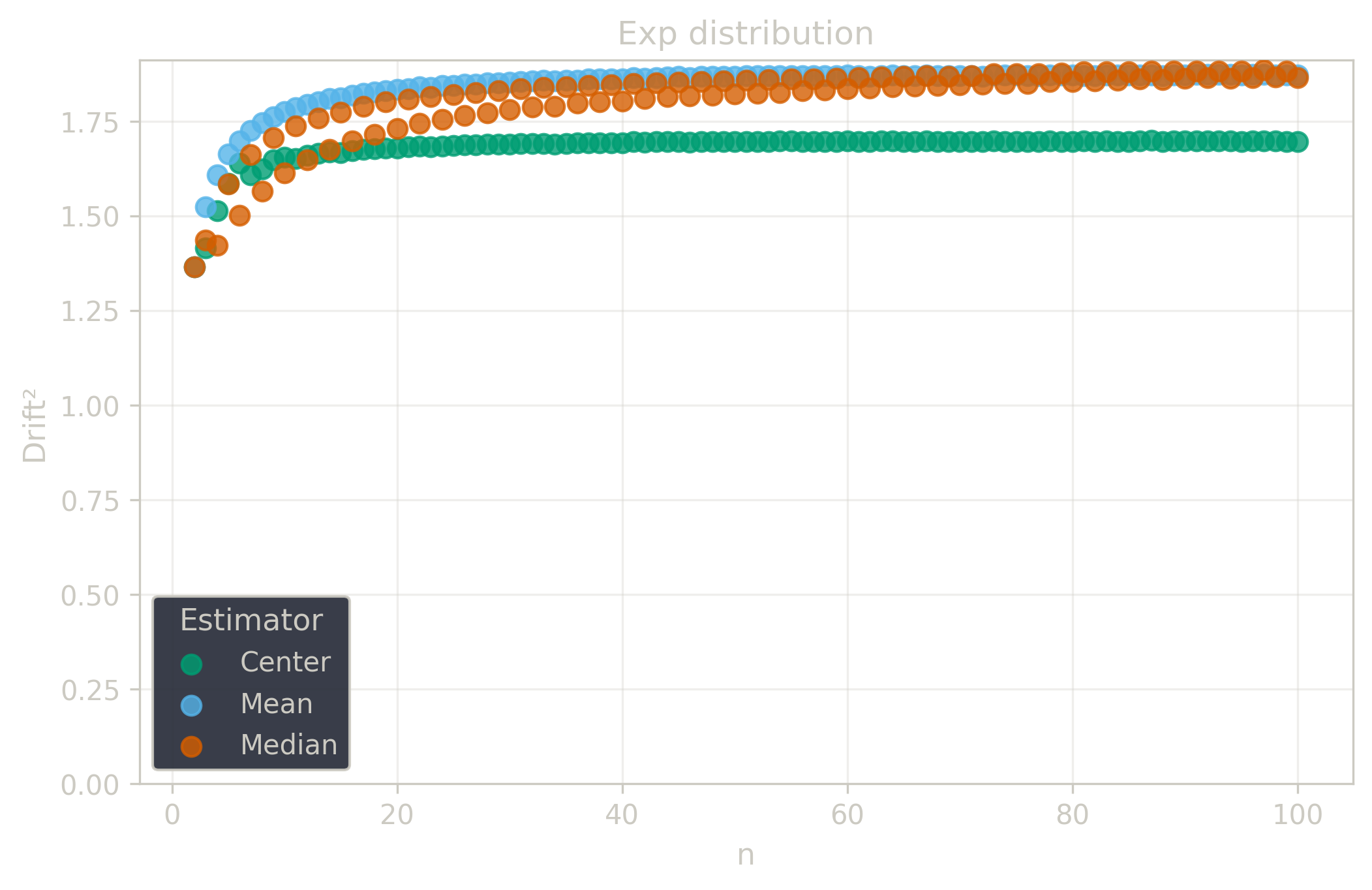
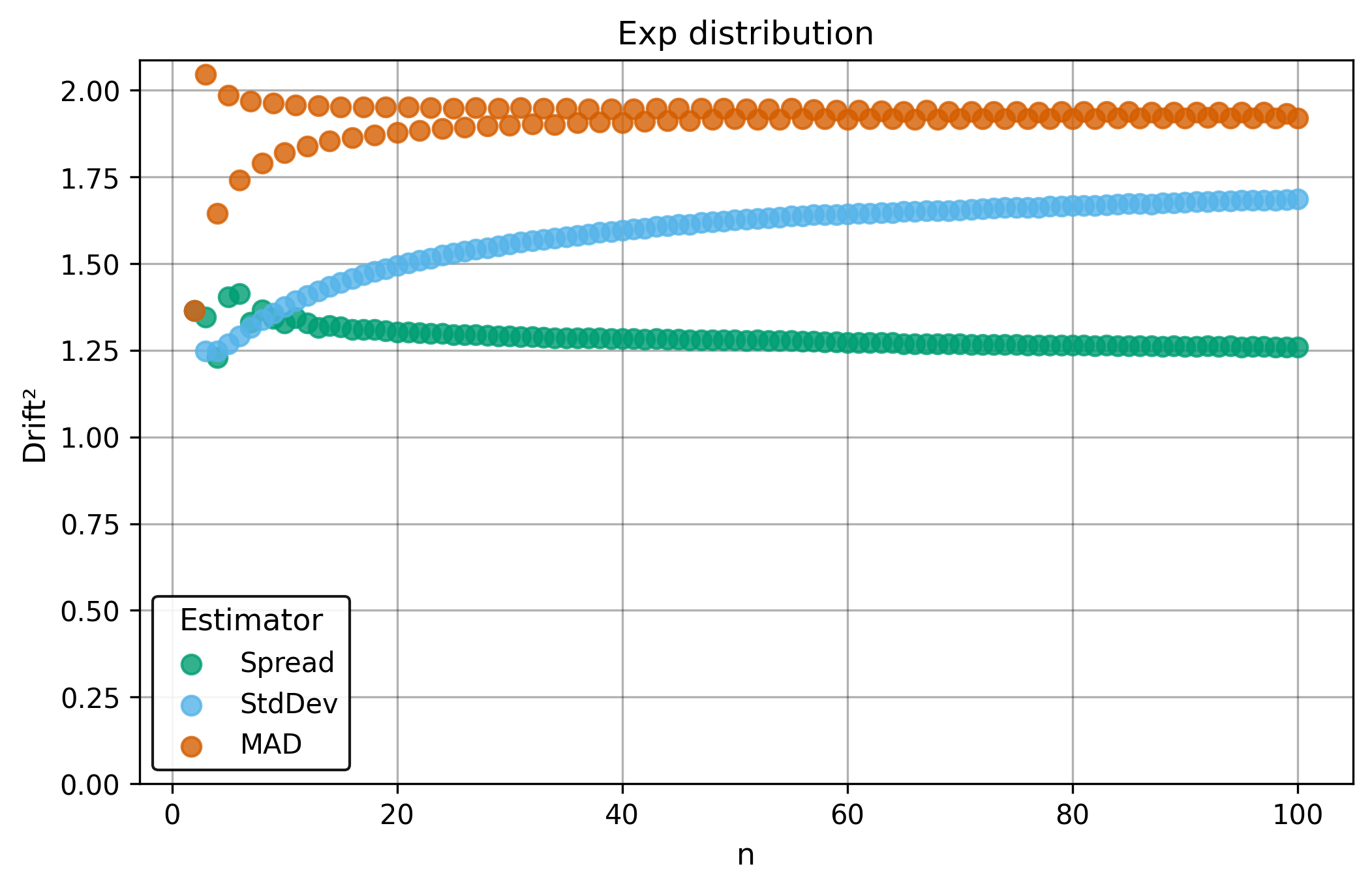
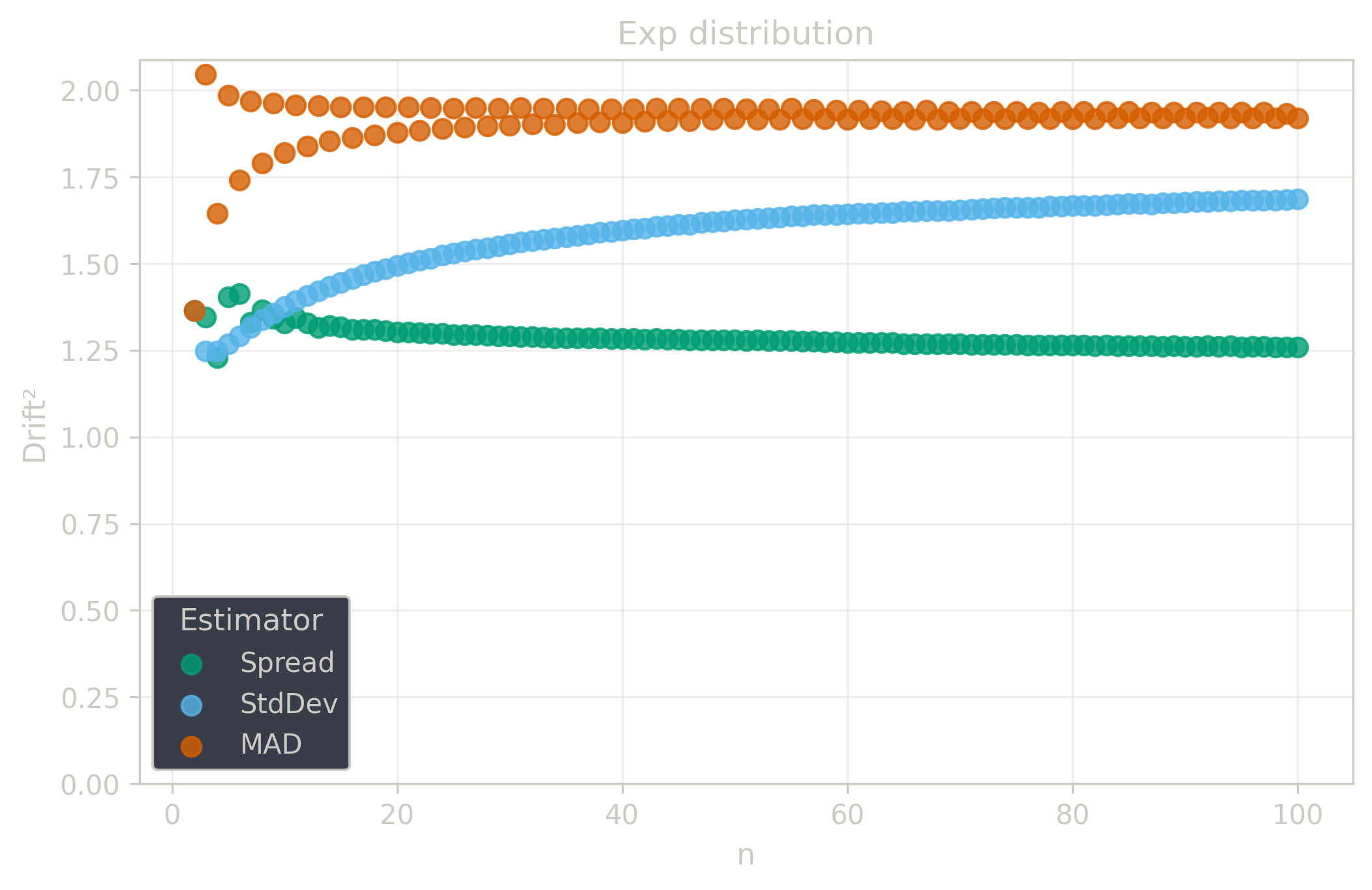
| $\Exp$ | 1.88 | 1.88 | 1.69 |
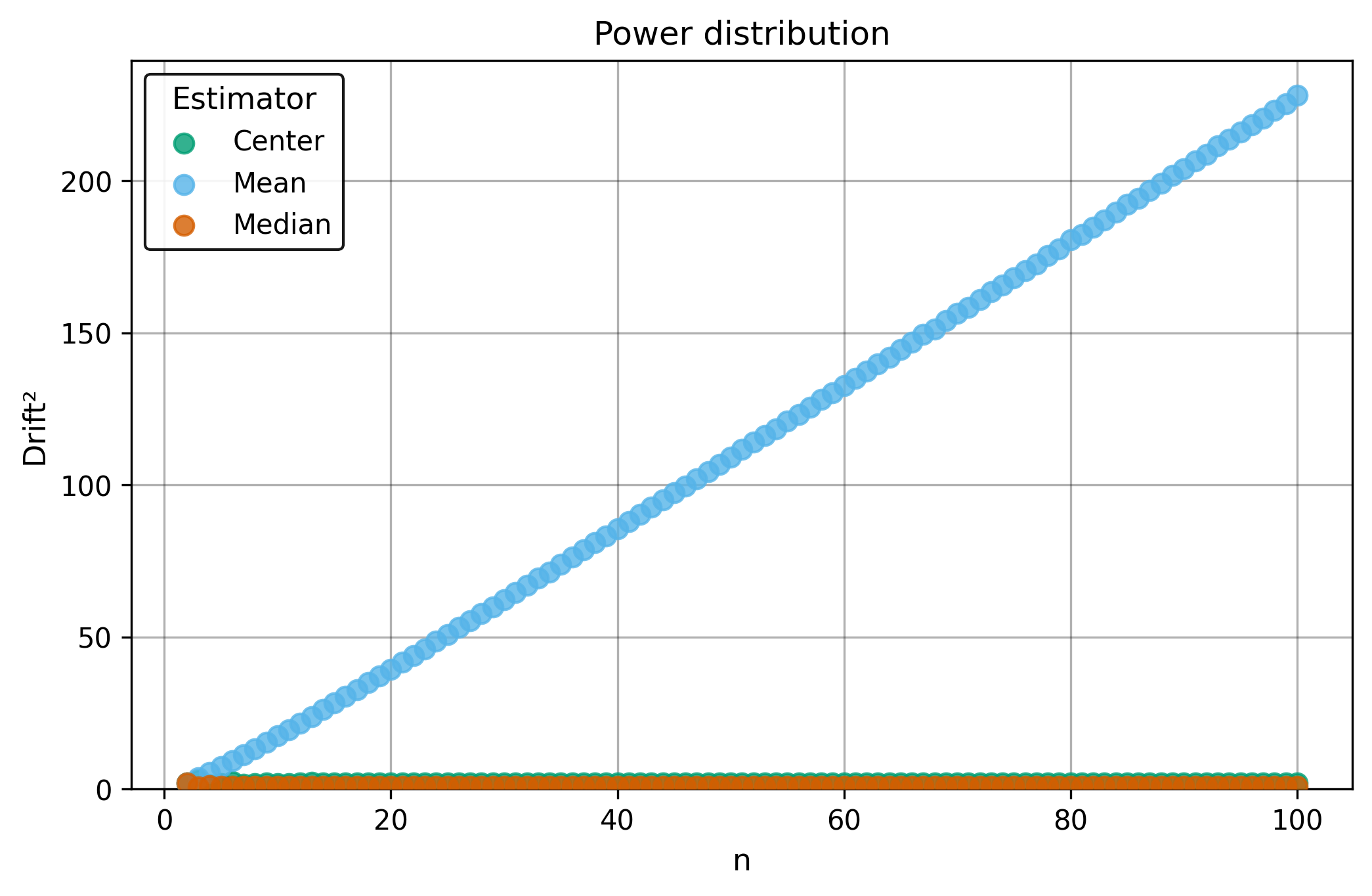
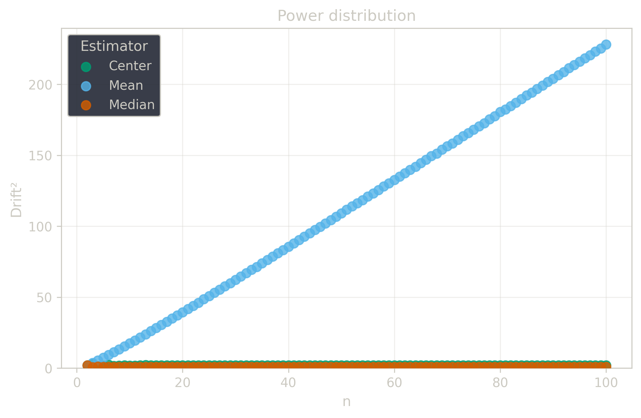
| $\Power$ | $\infty$ | 0.9 | 2.1 |
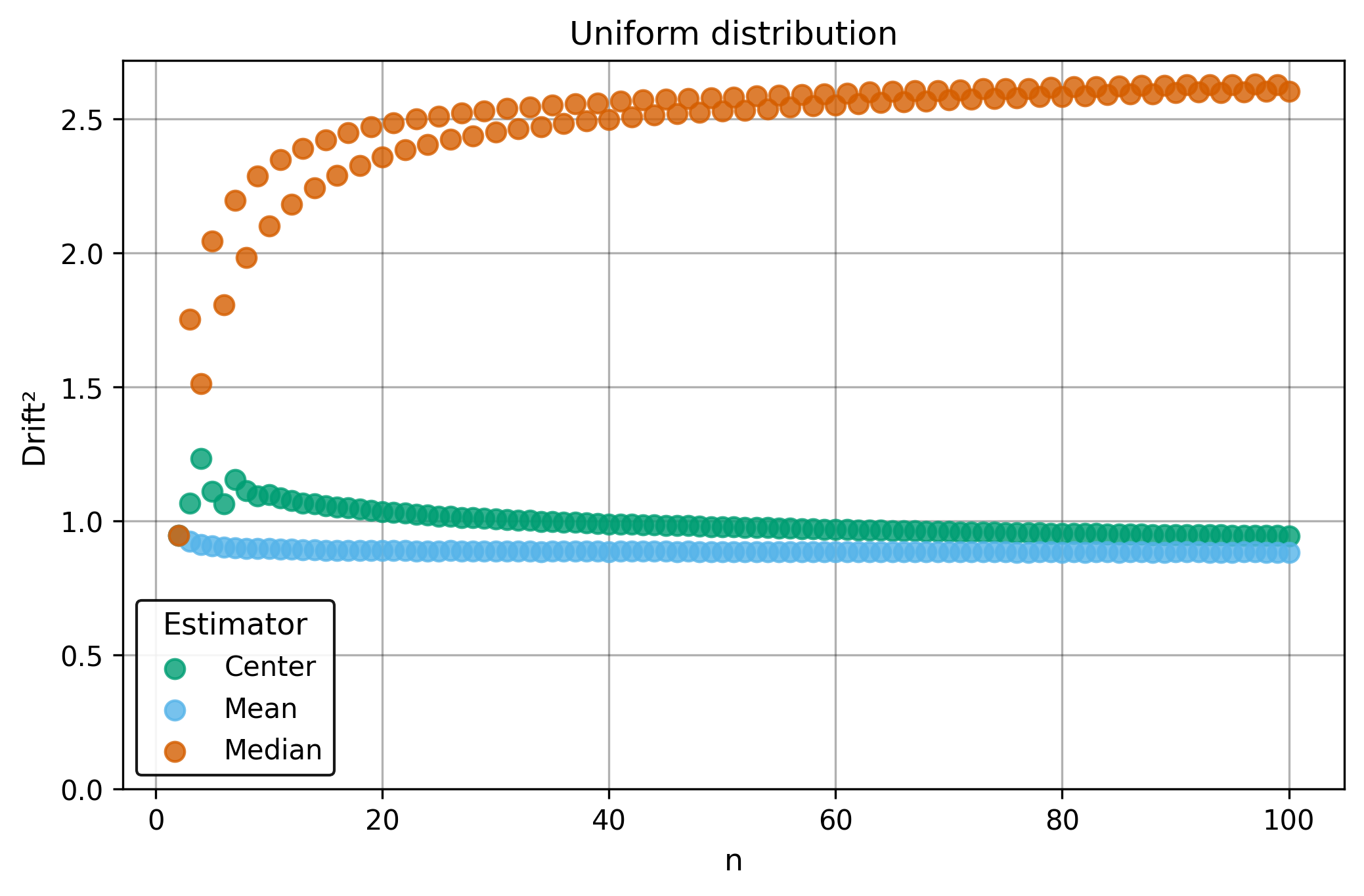
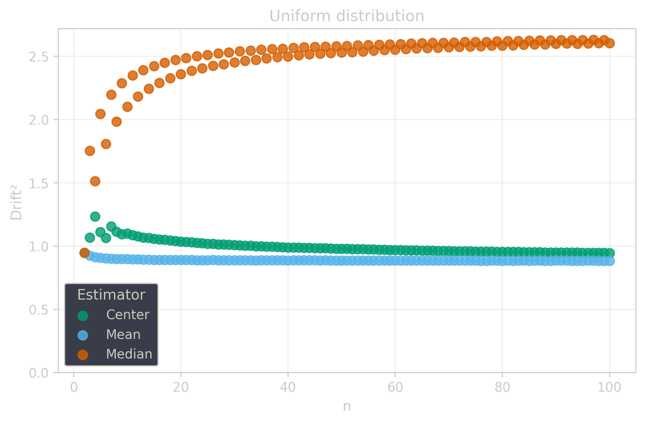
| $\Uniform$ | 0.88 | 2.60 | 0.94 |
Rescaled to $\Center$ (sample size adjustment factors):
| $\Mean$ | $\Median$ | $\Center$ | |
|---|---|---|---|
| $\Additive$ | 0.96 | 1.50 | 1.0 |
| $\Multiplic$ | 2.32 | 0.82 | 1.0 |
| $\Exp$ | 1.11 | 1.11 | 1.0 |
| $\Power$ | $\infty$ | 0.43 | 1.0 |
| $\Uniform$ | 0.936 | 2.77 | 1.0 |
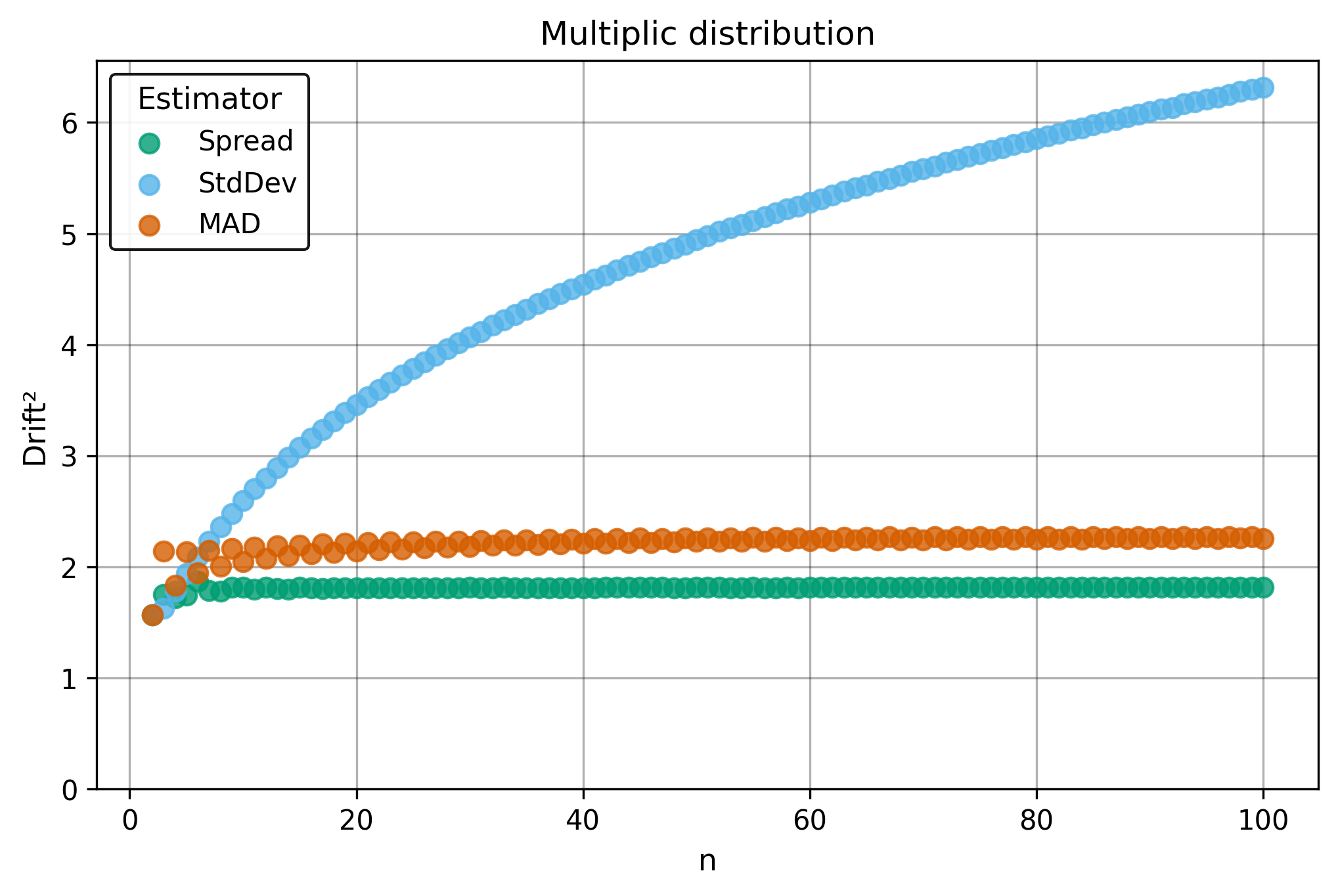
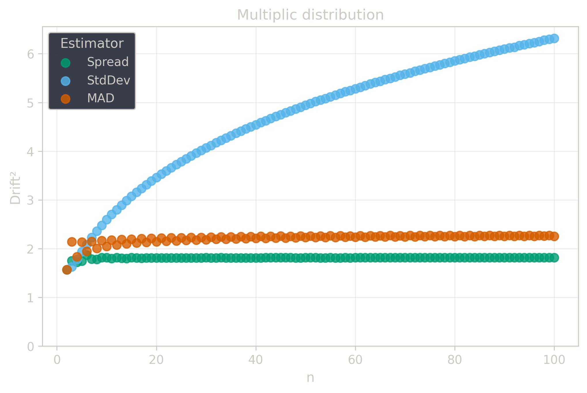
Squared Asymptotic Drift of Dispersion Estimators (values are approximated):
| $\StdDev$ | $\MAD$ | $\Spread$ | |
|---|---|---|---|
| $\Additive$ | 0.45 | 1.22 | 0.52 |
| $\Multiplic$ | $\infty$ | 2.26 | 1.81 |
| $\Exp$ | 1.69 | 1.92 | 1.26 |
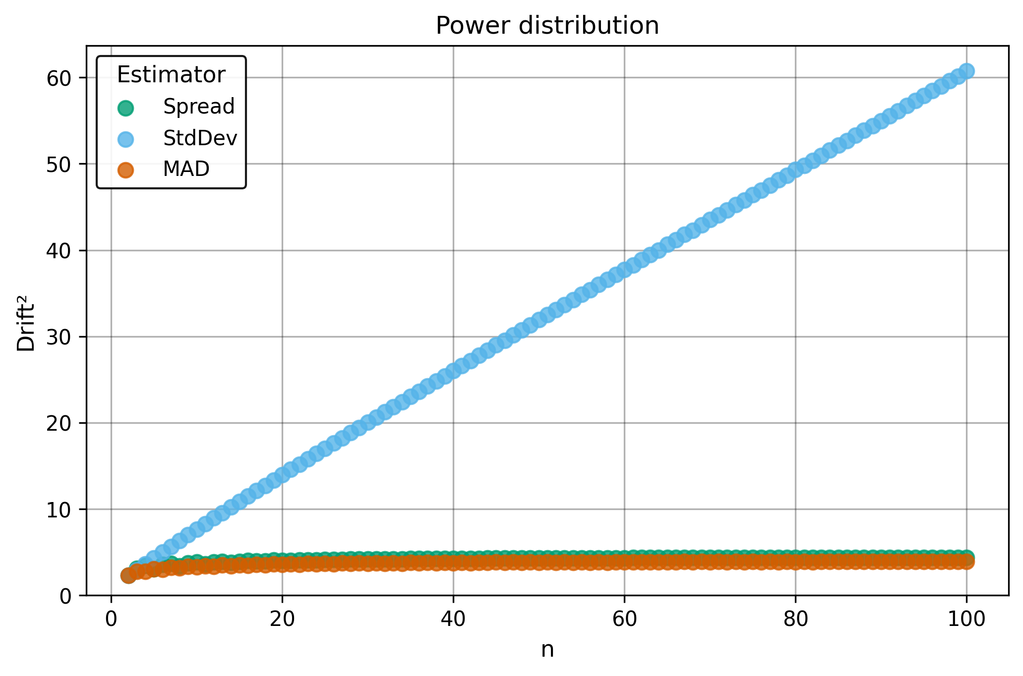
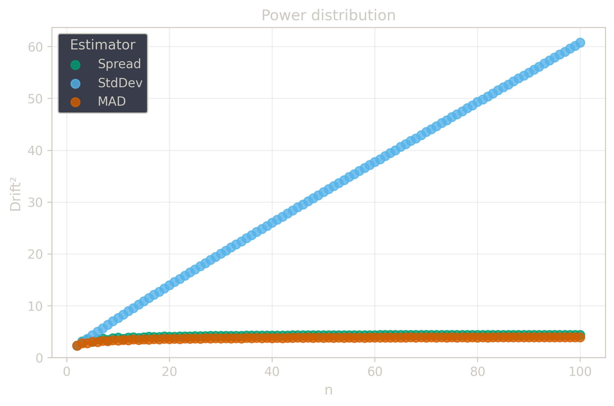
| $\Power$ | $\infty$ | 3.5 | 4.4 |
| $\Uniform$ | 0.18 | 0.90 | 0.43 |
Rescaled to $\Spread$ (sample size adjustment factors):
| $\StdDev$ | $\MAD$ | $\Spread$ | |
|---|---|---|---|
| $\Additive$ | 0.87 | 2.35 | 1.0 |
| $\Multiplic$ | $\infty$ | 1.25 | 1.0 |
| $\Exp$ | 1.34 | 1.52 | 1.0 |
| $\Power$ | $\infty$ | 0.80 | 1.0 |
| $\Uniform$ | 0.42 | 2.09 | 1.0 |
§4.3. Invariance
Invariance properties determine how estimators respond to data transformations. These properties are crucial for analysis design and interpretation:
- Location-invariant estimators are invariant to additive shifts: $T(\x+k)=T(\x)$
- Scale-invariant estimators are invariant to positive rescaling: $T(k \cdot \x)=T(\x)$ for $k>0$
- Equivariant estimators change predictably with transformations, maintaining relative relationships
Choosing estimators with appropriate invariance properties ensures that results remain meaningful across different measurement scales, units, and data transformations. For example, when comparing datasets collected with different instruments or protocols, location-invariant estimators eliminate the need for data centering, while scale-invariant estimators eliminate the need for normalization.
Location-invariance: An estimator $T$ is location-invariant if adding a constant to the measurements leaves the result unchanged:
$$ T(\x + k) = T(\x) $$$$ T(\x + k, \y + k) = T(\x, \y) $$Location-equivariance: An estimator $T$ is location-equivariant if it shifts with the data:
$$ T(\x + k) = T(\x) + k $$$$ T(\x + k_1, \y + k_2) = T(\x, \y) + f(k_1, k_2) $$Scale-invariance: An estimator $T$ is scale-invariant if multiplying by a positive constant leaves the result unchanged:
$$ T(k \cdot \x) = T(\x) \quad \text{for } k > 0 $$$$ T(k \cdot \x, k \cdot \y) = T(\x, \y) \quad \text{for } k > 0 $$Scale-equivariance: An estimator $T$ is scale-equivariant if it scales proportionally with the data:
$$ T(k \cdot \x) = k \cdot T(\x) \text{ or } |k| \cdot T(\x) \quad \text{for } k \neq 0 $$$$ T(k \cdot \x, k \cdot \y) = k \cdot T(\x, \y) \text{ or } |k| \cdot T(\x, \y) \quad \text{for } k \neq 0 $$| Location | Scale | |
|---|---|---|
| Center | Equivariant | Equivariant |
| Spread | Invariant | Equivariant |
| RelSpread | – | Invariant |
| Shift | Invariant | Equivariant |
| Ratio | – | Invariant |
| AvgSpread | Invariant | Equivariant |
| Disparity | Invariant | Invariant |
§5. Methodology
This chapter examines the methodological principles that guide the toolkit’s design and application.
§5.1. Desiderata
The toolkit consists of statistical procedures — practical methods that transform raw measurements into actionable insights and decisions. When practitioners face real-world problems involving data analysis, their success depends on selecting the right procedure for each specific situation. Convenient and efficient procedures have the following essential attributes:
- Usability. Procedures should feel natural to practitioners and minimize opportunities for misuse. They should be mathematically elegant yet accessible to readers with standard mathematical backgrounds. Implementation should be straightforward across programming languages. Like well-designed APIs, these procedures should follow intuitive design principles that reduce cognitive load.
- Reliability. Procedures should deliver consistent, trustworthy results, even in the presence of noise, data corruption, and extreme outliers.
- Applicability. Procedures should perform well across diverse contexts and sample sizes. They should handle the full spectrum of distributions commonly encountered in practice, from ideal theoretical models to data that deviates significantly from any assumed distribution.
This manual introduces a unified toolkit that aims to satisfy these properties and provide reliable rule-of-thumb procedures for everyday analytical tasks.
§5.2. From Assumptions to Conditions
Traditional statistical practice starts with model assumptions, then derives optimal procedures under those assumptions. This approach prioritizes mathematical convenience over practical application. Practitioners don’t know the distribution in advance, so they lack clear guidance on which procedure to choose by default.
Most traditional statistical procedures rely heavily on the $\Additive$ (‘Normal’) distribution and fail on real data because actual measurements contain outliers, exhibit skewness, or follow unknown distributions. When assumptions fail, procedures designed for those assumptions also fail.
This toolkit starts with procedures and tests how they perform under different distributional conditions. This approach reverses the traditional workflow: instead of deriving procedures from assumptions, we evaluate how each procedure performs across various distributions. This enables direct comparison and provides clear guidance on procedure selection based on known characteristics of the data source.
This procedure-first approach eliminates the need for complex mathematical derivations. All evaluations can be done numerically through Monte Carlo simulation. Generate samples from each distribution, apply each procedure, and measure the results. The numerical evidence directly shows which procedures work best under which conditions.
§5.3. From Statistical Efficiency to Drift
Statistical efficiency measures estimator precision. When multiple estimators target the same quantity, efficiency determines which provides more reliable results.
Efficiency measures how tightly estimates cluster around the true value across repeated samples. For an estimator $T$ applied to samples from distribution $X$, absolute efficiency is defined relative to the optimal estimator $T^*$:
$$ \text{Efficiency}(T, X) = \frac{\text{Var}[T^*(X_1, \ldots, X_n)]}{\text{Var}[T(X_1, \ldots, X_n)]} $$Relative efficiency compares two estimators by taking the ratio of their variances:
$$ \text{RelativeEfficiency}(T_1, T_2, X) = \frac{\text{Var}[T_2(X_1, \ldots, X_n)]}{\text{Var}[T_1(X_1, \ldots, X_n)]} $$Under $\Additive$ (‘Normal’) distributions, this approach works well. The sample mean achieves optimal efficiency, while the median operates at roughly 64% efficiency.
However, this variance-based definition creates four critical limitations:
- Absolute efficiency requires knowing the optimal estimator, which is often difficult to determine. For many distributions, deriving the minimum-variance unbiased estimator requires complex mathematical analysis. Without this reference point, absolute efficiency cannot be computed.
- Relative efficiency only compares estimator pairs, preventing systematic evaluation. This limits understanding of how multiple estimators perform relative to each other. Practitioners cannot rank estimators comprehensively or evaluate individual performance in isolation.
- The approach depends on variance calculations that break down when variance becomes infinite or when distributions have heavy tails. Many real-world distributions, such as those with power-law tails, exhibit infinite variance. When the variance is undefined, efficiency comparisons become impossible.
- Variance is not robust to outliers, which can corrupt efficiency calculations. A single extreme observation can greatly inflate variance estimates. This sensitivity can make efficient estimators look inefficient and vice versa.
The $\Drift$ concept provides a robust alternative. Drift measures estimator precision using $\Spread$ instead of variance, providing reliable comparisons across a wide range of distributions.
For an average estimator $T$, random variable $X$, and sample size $n$:
$$ \AvgDrift(T, X, n) = \frac{\sqrt{n}\,\Spread\big[T(X_1, \ldots, X_n)\big]}{\Spread[X]} $$This formula measures estimator variability compared to data variability. $\Spread\big[T(X_1, \ldots, X_n)\big]$ captures the median absolute difference between estimates across repeated samples. Multiplying by $\sqrt{n}$ removes sample size dependency, making drift values comparable across different sample sizes. Dividing by $\Spread[X]$ creates a scale-free measure that provides consistent drift values across different distribution parameters and measurement units.
Dispersion estimators use a parallel formulation:
$$ \DispDrift(T, X, n) = \sqrt{n}\,\RelSpread\big[T(X_1, \ldots, X_n)\big] $$Here $\RelSpread$ normalizes by the estimator’s typical value for fair comparison.
Drift offers four key advantages:
- For estimators with $\sqrt{n}$ convergence rates, drift remains finite and comparable across distributions; for heavier tails, drift may diverge, flagging estimator instability.
- It provides absolute precision measures rather than only pairwise comparisons.
- The robust $\Spread$ foundation resists outlier distortion that corrupts variance-based calculations.
- The $\sqrt{n}$ normalization makes drift values comparable across different sample sizes, enabling direct comparison of estimator performance regardless of sample size.
Under $\Additive$ (‘Normal’) conditions, drift matches traditional efficiency. The sample mean achieves drift near 1.0; the median achieves drift around 1.25. This consistency validates drift as a proper generalization of efficiency that extends to realistic data conditions where traditional efficiency fails.
When switching from one estimator to another while maintaining the same precision, the required sample size adjustment follows:
$$ n_{\text{new}} = n_{\text{original}} \cdot \frac{\Drift^2(T_2, X)}{\Drift^2(T_1, X)} $$This applies when estimator $T_1$ has lower drift than $T_2$.
The ratio of squared drifts determines the data requirement change. If $T_2$ has drift 1.5 times higher than $T_1$, then $T_2$ requires $(1.5)^2 = 2.25$ times more data to match $T_1$’s precision. Conversely, switching to a more precise estimator allows smaller sample sizes.
For asymptotic analysis, $\Drift(T, X)$ denotes the limiting value as $n \to \infty$. With a baseline estimator, rescaled drift values enable direct comparisons:
$$ \Drift_{\textrm{baseline}}(T, X) = \frac{\Drift(T, X)}{\Drift\big(T_{\textrm{baseline}}, X\big)} $$The standard drift definition assumes $\sqrt{n}$ convergence rates typical under $\Additive$ (‘Normal’) conditions. For broader applicability, drift generalizes to:
$$ \AvgDrift(T, X, n) = \frac{n^{\textrm{instability}}\,\Spread\big[T(X_1, \ldots, X_n)\big]}{\Spread[X]} $$$$ \DispDrift(T, X, n) = n^{\textrm{instability}}\,\RelSpread\big[T(X_1, \ldots, X_n)\big] $$The instability parameter adapts to estimator convergence rates. The toolkit uses $\textrm{instability} = 1/2$ throughout because this choice provides natural intuition and mental representation for the $\Additive$ (‘Normal’) distribution. Rather than introduce additional complexity through variable instability parameters, the fixed $\sqrt{n}$ scaling offers practical convenience while maintaining theoretical rigor for the distribution classes most common in applications.
§6. Algorithms
This chapter describes the core algorithms that power the robust estimators in the toolkit. Both algorithms solve a fundamental computational challenge: how to efficiently find medians within large collections of derived values without materializing the entire collection in memory.
§6.1. Fast Center
The $\Center$ estimator computes the median of all pairwise averages from a sample. Given a dataset $x = (x_1, x_2, \ldots, x_n)$, this estimator is defined as:
$$ \Center(\x) = \underset{1 \leq i \leq j \leq n}{\Median} \left(\frac{x_i + x_j}{2} \right) $$A direct implementation would generate all $\frac{n(n+1)}{2}$ pairwise averages and sort them. With $n = 10,000$, this approach creates approximately 50 million values, requiring quadratic memory and $O(n^2 \log n)$ time.
The breakthrough came in 1984 when John Monahan developed an algorithm that reduces expected complexity to $O(n \log n)$ while using only linear memory (see monahan1984). The algorithm exploits the inherent structure in pairwise sums rather than computing them explicitly. After sorting the values $x_1 \leq x_2 \leq \cdots \leq x_n$, the algorithm considers the implicit upper triangular matrix $M$ where $M_{i,j} = x_i + x_j$ for $i \leq j$. This matrix has a crucial property: each row and column is sorted in non-decreasing order, enabling efficient median selection without storing the matrix.
Rather than sorting all pairwise sums, the algorithm uses a selection approach similar to quickselect. It maintains search bounds for each matrix row and iteratively narrows the search space. For each row $i$, the algorithm tracks active column indices from $i+1$ to $n$, defining which pairwise sums remain candidates for the median. It selects a candidate sum as a pivot using randomized selection from active matrix elements, then counts how many pairwise sums fall below the pivot. Because both rows and columns are sorted, this counting takes only $O(n)$ time using a two-pointer sweep from the matrix’s upper-right corner.
The median corresponds to rank $k = \lfloor \frac{N+1}{2} \rfloor$ where $N = \frac{n(n+1)}{2}$. If fewer than $k$ sums lie below the pivot, the median must be larger; if more than $k$ sums lie below the pivot, the median must be smaller. Based on this comparison, the algorithm eliminates portions of each row that cannot contain the median, shrinking the active search space while preserving the true median.
Real data often contain repeated values, which can cause the selection process to stall. When the algorithm detects no progress between iterations, it switches to a midrange strategy: find the smallest and largest pairwise sums still in the search space, then use their average as the next pivot. If the minimum equals the maximum, all remaining candidates are identical and the algorithm terminates. This tie-breaking mechanism ensures reliable convergence with discrete or duplicated data.
The algorithm achieves $O(n \log n)$ time complexity through linear partitioning (each pivot evaluation requires only $O(n)$ operations) and logarithmic iterations (randomized pivot selection leads to expected $O(\log n)$ iterations, similar to quickselect). The algorithm maintains only row bounds and counters, using $O(n)$ additional space. This matches the complexity of sorting a single array while avoiding the quadratic memory and time explosion of computing all pairwise combinations.
▼ FastCenter.cs
namespace Pragmastat.Algorithms;

internal static class FastCenter
{
  /// <summary>
  /// ACM Algorithm 616: fast computation of the Hodges-Lehmann location estimator
  /// </summary>
  /// <remarks>
  /// Computes the median of all pairwise averages (xi + xj)/2 efficiently.
  /// See: John F Monahan, "Algorithm 616: fast computation of the Hodges-Lehmann location estimator"
  /// (1984) DOI: 10.1145/1271.319414
  /// </remarks>
  /// <param name="values">A sorted sample of values</param>
  /// <param name="random">Random number generator</param>
  /// <param name="isSorted">If values are sorted</param>
  /// <returns>Exact center value (Hodges-Lehmann estimator)</returns>
  public static double Estimate(IReadOnlyList<double> values, Random? random = null, bool isSorted = false)
  {
    int n = values.Count;
    if (n == 1) return values[0];
    if (n == 2) return (values[0] + values[1]) / 2;
    random ??= new Random();
    if (!isSorted)
      values = values.OrderBy(x => x).ToList();

    // Calculate target median rank(s) among all pairwise sums
    long totalPairs = (long)n * (n + 1) / 2;
    long medianRankLow = (totalPairs + 1) / 2; // For odd totalPairs, this is the median
    long medianRankHigh =
      (totalPairs + 2) / 2; // For even totalPairs, average of ranks medianRankLow and medianRankHigh

    // Initialize search bounds for each row in the implicit matrix
    long[] leftBounds = new long[n];
    long[] rightBounds = new long[n];
    long[] partitionCounts = new long[n];

    for (int i = 0; i < n; i++)
    {
      leftBounds[i] = i + 1; // Row i can pair with columns [i+1..n] (1-based indexing)
      rightBounds[i] = n; // Initially, all columns are available
    }

    // Start with a good pivot: sum of middle elements (handles both odd and even n)
    double pivot = values[(n - 1) / 2] + values[n / 2];
    long activeSetSize = totalPairs;
    long previousCount = 0;

    while (true)
    {
      // === PARTITION STEP ===
      // Count pairwise sums less than current pivot
      long countBelowPivot = 0;
      long currentColumn = n;

      for (int row = 1; row <= n; row++)
      {
        partitionCounts[row - 1] = 0;

        // Move left from current column until we find sums < pivot
        // This exploits the sorted nature of the matrix
        while (currentColumn >= row && values[row - 1] + values[(int)currentColumn - 1] >= pivot)
          currentColumn--;

        // Count elements in this row that are < pivot
        if (currentColumn >= row)
        {
          long elementsBelow = currentColumn - row + 1;
          partitionCounts[row - 1] = elementsBelow;
          countBelowPivot += elementsBelow;
        }
      }

      // === CONVERGENCE CHECK ===
      // If no progress, we have ties - break them using midrange strategy
      if (countBelowPivot == previousCount)
      {
        double minActiveSum = double.MaxValue;
        double maxActiveSum = double.MinValue;

        // Find the range of sums still in the active search space
        for (int i = 0; i < n; i++)
        {
          if (leftBounds[i] > rightBounds[i]) continue; // Skip empty rows

          double rowValue = values[i];
          double smallestInRow = values[(int)leftBounds[i] - 1] + rowValue;
          double largestInRow = values[(int)rightBounds[i] - 1] + rowValue;

          minActiveSum = Min(minActiveSum, smallestInRow);
          maxActiveSum = Max(maxActiveSum, largestInRow);
        }

        pivot = (minActiveSum + maxActiveSum) / 2;
        if (pivot <= minActiveSum || pivot > maxActiveSum) pivot = maxActiveSum;

        // If all remaining values are identical, we're done
        if (minActiveSum == maxActiveSum || activeSetSize <= 2)
          return pivot / 2;

        continue;
      }

      // === TARGET CHECK ===
      // Check if we've found the median rank(s)
      bool atTargetRank = countBelowPivot == medianRankLow || countBelowPivot == medianRankHigh - 1;
      if (atTargetRank)
      {
        // Find the boundary values: largest < pivot and smallest >= pivot
        double largestBelowPivot = double.MinValue;
        double smallestAtOrAbovePivot = double.MaxValue;

        for (int i = 1; i <= n; i++)
        {
          long countInRow = partitionCounts[i - 1];
          double rowValue = values[i - 1];
          long totalInRow = n - i + 1;

          // Find largest sum in this row that's < pivot
          if (countInRow > 0)
          {
            long lastBelowIndex = i + countInRow - 1;
            double lastBelowValue = rowValue + values[(int)lastBelowIndex - 1];
            largestBelowPivot = Max(largestBelowPivot, lastBelowValue);
          }

          // Find smallest sum in this row that's >= pivot
          if (countInRow < totalInRow)
          {
            long firstAtOrAboveIndex = i + countInRow;
            double firstAtOrAboveValue = rowValue + values[(int)firstAtOrAboveIndex - 1];
            smallestAtOrAbovePivot = Min(smallestAtOrAbovePivot, firstAtOrAboveValue);
          }
        }

        // Calculate final result based on whether we have odd or even number of pairs
        if (medianRankLow < medianRankHigh)
        {
          // Even total: average the two middle values
          return (smallestAtOrAbovePivot + largestBelowPivot) / 4;
        }
        else
        {
          // Odd total: return the single middle value
          bool needLargest = countBelowPivot == medianRankLow;
          return (needLargest ? largestBelowPivot : smallestAtOrAbovePivot) / 2;
        }
      }

      // === UPDATE BOUNDS ===
      // Narrow the search space based on partition result
      if (countBelowPivot < medianRankLow)
      {
        // Too few values below pivot - eliminate smaller values, search higher
        for (int i = 0; i < n; i++)
          leftBounds[i] = i + partitionCounts[i] + 1;
      }
      else
      {
        // Too many values below pivot - eliminate larger values, search lower
        for (int i = 0; i < n; i++)
          rightBounds[i] = i + partitionCounts[i];
      }

      // === PREPARE NEXT ITERATION ===
      previousCount = countBelowPivot;

      // Recalculate how many elements remain in the active search space
      activeSetSize = 0;
      for (int i = 0; i < n; i++)
      {
        long rowSize = rightBounds[i] - leftBounds[i] + 1;
        activeSetSize += Max(0, rowSize);
      }

      // Choose next pivot based on remaining active set size
      if (activeSetSize > 2)
      {
        // Use randomized row median strategy for efficiency
        // Handle large activeSetSize by using double precision for random selection
        double randomFraction = random.NextDouble();
        long targetIndex = (long)(randomFraction * activeSetSize);
        int selectedRow = 0;

        // Find which row contains the target index
        long cumulativeSize = 0;
        for (int i = 0; i < n; i++)
        {
          long rowSize = Max(0, rightBounds[i] - leftBounds[i] + 1);
          if (targetIndex < cumulativeSize + rowSize)
          {
            selectedRow = i;
            break;
          }

          cumulativeSize += rowSize;
        }

        // Use median element of the selected row as pivot
        long medianColumnInRow = (leftBounds[selectedRow] + rightBounds[selectedRow]) / 2;
        pivot = values[selectedRow] + values[(int)medianColumnInRow - 1];
      }
      else
      {
        // Few elements remain - use midrange strategy
        double minRemainingSum = double.MaxValue;
        double maxRemainingSum = double.MinValue;

        for (int i = 0; i < n; i++)
        {
          if (leftBounds[i] > rightBounds[i]) continue; // Skip empty rows

          double rowValue = values[i];
          double minInRow = values[(int)leftBounds[i] - 1] + rowValue;
          double maxInRow = values[(int)rightBounds[i] - 1] + rowValue;

          minRemainingSum = Min(minRemainingSum, minInRow);
          maxRemainingSum = Max(maxRemainingSum, maxInRow);
        }

        pivot = (minRemainingSum + maxRemainingSum) / 2;
        if (pivot <= minRemainingSum || pivot > maxRemainingSum)
          pivot = maxRemainingSum;

        if (minRemainingSum == maxRemainingSum)
          return pivot / 2;
      }
    }
  }
}
§6.2. Fast Spread
The $\Spread$ estimator computes the median of all pairwise absolute differences. Given a sample $x = (x_1, x_2, \ldots, x_n)$, this estimator is defined as:
$$ \Spread(\x) = \underset{1 \leq i < j \leq n}{\Median} |x_i - x_j| $$Like $\Center$, computing $\Spread$ naively requires generating all $\frac{n(n-1)}{2}$ pairwise differences, sorting them, and finding the median — a quadratic approach that becomes computationally prohibitive for large datasets.
The same structural principles that accelerate $\Center$ computation also apply to pairwise differences, yielding an exact $O(n \log n)$ algorithm. After sorting the input to obtain $y_1 \leq y_2 \leq \cdots \leq y_n$, all pairwise absolute differences $|x_i - x_j|$ with $i < j$ become positive differences $y_j - y_i$. This allows considering the implicit upper triangular matrix $D$ where $D_{i,j} = y_j - y_i$ for $i < j$. This matrix has a crucial structural property: for a fixed row $i$, differences increase monotonically, while for a fixed column $j$, differences decrease as $i$ increases. This sorted structure enables linear-time counting of elements below any threshold.
The algorithm applies Monahan’s selection strategy, adapted for differences rather than sums. For each row $i$, it tracks active column indices representing differences still under consideration, initially spanning columns $i+1$ through $n$. It chooses candidate differences from the active set using weighted random row selection, maintaining expected logarithmic convergence while avoiding expensive pivot computations. For any pivot value $p$, the number of differences falling below $p$ is counted using a single sweep; the monotonic structure ensures this counting requires only $O(n)$ operations. While counting, the largest difference below $p$ and the smallest difference at or above $p$ are maintained— these boundary values become the exact answer when the target rank is reached.
The algorithm naturally handles both odd and even cases. For an odd number of differences, it returns the single middle element when the count exactly hits the median rank. For an even number of differences, it returns the average of the two middle elements; boundary tracking during counting provides both values simultaneously. Unlike approximation methods, this algorithm returns the precise median of all pairwise differences; randomness affects only performance, not correctness.
The algorithm includes the same stall-handling mechanisms as the center algorithm. It tracks whether the count below the pivot changes between iterations; when progress stalls due to tied values, it computes the range of remaining active differences and pivots to their midrange. This midrange strategy ensures convergence even with highly discrete data or datasets with many identical values.
Several optimizations make the implementation practical for production use. A global column pointer that never moves backward during counting exploits the matrix structure to avoid redundant comparisons. Exact boundary values are captured during each counting pass, eliminating the need for additional searches when the target rank is reached. Using only $O(n)$ additional space for row bounds and counters, the algorithm achieves $O(n \log n)$ time complexity with minimal memory overhead, making robust scale estimation practical for large datasets.
▼ FastSpread.cs
namespace Pragmastat.Algorithms;

internal static class FastSpread
{
  /// <summary>
  /// Shamos "Spread".  Expected O(n log n) time, O(n) extra space. Exact.
  /// </summary>
  public static double Estimate(IReadOnlyList<double> values, Random? random = null, bool isSorted = false)
  {
    int n = values.Count;
    if (n <= 1) return 0;
    if (n == 2) return Abs(values[1] - values[0]);
    random ??= new Random();

    // Prepare a sorted working copy.
    double[] a = isSorted ? CopySorted(values) : EnsureSorted(values);

    // Total number of pairwise differences with i < j
    long N = (long)n * (n - 1) / 2;
    long kLow = (N + 1) / 2; // 1-based rank of lower middle
    long kHigh = (N + 2) / 2; // 1-based rank of upper middle

    // Per-row active bounds over columns j (0-based indices).
    // Row i allows j in [i+1, n-1] initially.
    int[] L = new int[n];
    int[] R = new int[n];
    long[] rowCounts = new long[n]; // # of elements in row i that are < pivot (for current partition)

    for (int i = 0; i < n; i++)
    {
      L[i] = Min(i + 1, n); // n means empty
      R[i] = n - 1; // inclusive
      if (L[i] > R[i])
      {
        L[i] = 1;
        R[i] = 0;
      } // mark empty
    }

    // A reasonable initial pivot: a central gap
    double pivot = a[n / 2] - a[(n - 1) / 2];

    long prevCountBelow = -1;

    while (true)
    {
      // === PARTITION: count how many differences are < pivot; also track boundary neighbors ===
      long countBelow = 0;
      double largestBelow = double.NegativeInfinity; // max difference < pivot
      double smallestAtOrAbove = double.PositiveInfinity; // min difference >= pivot

      int j = 1; // global two-pointer (non-decreasing across rows)
      for (int i = 0; i < n - 1; i++)
      {
        if (j < i + 1) j = i + 1;
        while (j < n && a[j] - a[i] < pivot) j++;

        long cntRow = j - (i + 1);
        if (cntRow < 0) cntRow = 0;
        rowCounts[i] = cntRow;
        countBelow += cntRow;

        // boundary elements for this row
        if (cntRow > 0)
        {
          // last < pivot in this row is (j-1)
          double candBelow = a[j - 1] - a[i];
          if (candBelow > largestBelow) largestBelow = candBelow;
        }

        if (j < n)
        {
          double candAtOrAbove = a[j] - a[i];
          if (candAtOrAbove < smallestAtOrAbove) smallestAtOrAbove = candAtOrAbove;
        }
      }

      // === TARGET CHECK ===
      // If we've split exactly at the middle, we can return using the boundaries we just found.
      bool atTarget =
        (countBelow == kLow) || // lower middle is the largest < pivot
        (countBelow == (kHigh - 1)); // upper middle is the smallest >= pivot

      if (atTarget)
      {
        if (kLow < kHigh)
        {
          // Even N: average the two central order stats.
          return 0.5 * (largestBelow + smallestAtOrAbove);
        }
        else
        {
          // Odd N: pick the single middle depending on which side we hit.
          bool needLargest = (countBelow == kLow);
          return needLargest ? largestBelow : smallestAtOrAbove;
        }
      }

      // === STALL HANDLING (ties / no progress) ===
      if (countBelow == prevCountBelow)
      {
        // Compute min/max remaining difference in the ACTIVE set and pivot to their midrange.
        double minActive = double.PositiveInfinity;
        double maxActive = double.NegativeInfinity;
        long active = 0;

        for (int i = 0; i < n - 1; i++)
        {
          int Li = L[i], Ri = R[i];
          if (Li > Ri) continue;

          double rowMin = a[Li] - a[i];
          double rowMax = a[Ri] - a[i];
          if (rowMin < minActive) minActive = rowMin;
          if (rowMax > maxActive) maxActive = rowMax;
          active += (Ri - Li + 1);
        }

        if (active <= 0)
        {
          // No active candidates left: the only consistent answer is the boundary implied by counts.
          // Fall back to neighbors from this partition.
          if (kLow < kHigh) return 0.5 * (largestBelow + smallestAtOrAbove);
          return (countBelow >= kLow) ? largestBelow : smallestAtOrAbove;
        }

        if (maxActive <= minActive) return minActive; // all remaining equal

        double mid = 0.5 * (minActive + maxActive);
        pivot = (mid > minActive && mid <= maxActive) ? mid : maxActive;
        prevCountBelow = countBelow;
        continue;
      }

      // === SHRINK ACTIVE WINDOW ===
// --- SHRINK ACTIVE WINDOW (fixed) ---
      if (countBelow < kLow)
      {
        // Need larger differences: discard all strictly below pivot.
        for (int i = 0; i < n - 1; i++)
        {
          // First j with a[j] - a[i] >= pivot is j = i + 1 + cntRow (may be n => empty row)
          int newL = i + 1 + (int)rowCounts[i];
          if (newL > L[i]) L[i] = newL; // do NOT clamp; allow L[i] == n to mean empty
          if (L[i] > R[i])
          {
            L[i] = 1;
            R[i] = 0;
          } // mark empty
        }
      }
      else
      {
        // Too many below: keep only those strictly below pivot.
        for (int i = 0; i < n - 1; i++)
        {
          // Last j with a[j] - a[i] < pivot is j = i + cntRow  (not cntRow-1!)
          int newR = i + (int)rowCounts[i];
          if (newR < R[i]) R[i] = newR; // shrink downward to the true last-below
          if (R[i] < i + 1)
          {
            L[i] = 1;
            R[i] = 0;
          } // empty row if none remain
        }
      }

      prevCountBelow = countBelow;

      // === CHOOSE NEXT PIVOT FROM ACTIVE SET (weighted random row, then row median) ===
      long activeSize = 0;
      for (int i = 0; i < n - 1; i++)
      {
        if (L[i] <= R[i]) activeSize += (R[i] - L[i] + 1);
      }

      if (activeSize <= 2)
      {
        // Few candidates left: return midrange of remaining exactly.
        double minRem = double.PositiveInfinity, maxRem = double.NegativeInfinity;
        for (int i = 0; i < n - 1; i++)
        {
          if (L[i] > R[i]) continue;
          double lo = a[L[i]] - a[i];
          double hi = a[R[i]] - a[i];
          if (lo < minRem) minRem = lo;
          if (hi > maxRem) maxRem = hi;
        }

        if (activeSize <= 0) // safety net; fall back to boundary from last partition
        {
          if (kLow < kHigh) return 0.5 * (largestBelow + smallestAtOrAbove);
          return (countBelow >= kLow) ? largestBelow : smallestAtOrAbove;
        }

        if (kLow < kHigh) return 0.5 * (minRem + maxRem);
        return (Abs((kLow - 1) - countBelow) <= Abs(countBelow - kLow)) ? minRem : maxRem;
      }
      else
      {
        long t = NextIndex(random, activeSize); // 0..activeSize-1
        long acc = 0;
        int row = 0;
        for (; row < n - 1; row++)
        {
          if (L[row] > R[row]) continue;
          long size = R[row] - L[row] + 1;
          if (t < acc + size) break;
          acc += size;
        }

        // Median column of the selected row
        int col = (L[row] + R[row]) >> 1;
        pivot = a[col] - a[row];
      }
    }
  }
  // --- Helpers ---

  private static double[] CopySorted(IReadOnlyList<double> values)
  {
    var a = new double[values.Count];
    for (int i = 0; i < a.Length; i++)
    {
      double v = values[i];
      if (double.IsNaN(v)) throw new ArgumentException("NaN not allowed.", nameof(values));
      a[i] = v;
    }

    Array.Sort(a);
    return a;
  }

  private static double[] EnsureSorted(IReadOnlyList<double> values)
  {
    // Trust caller; still copy to array for fast indexed access.
    var a = new double[values.Count];
    for (int i = 0; i < a.Length; i++)
    {
      double v = values[i];
      if (double.IsNaN(v)) throw new ArgumentException("NaN not allowed.", nameof(values));
      a[i] = v;
    }

    return a;
  }

  private static long NextIndex(Random rng, long limitExclusive)
  {
    // Uniform 0..limitExclusive-1 even for large ranges.
    // Use rejection sampling for correctness.
    ulong uLimit = (ulong)limitExclusive;
    if (uLimit <= int.MaxValue)
    {
      return rng.Next((int)uLimit);
    }

    while (true)
    {
      ulong u = ((ulong)(uint)rng.Next() << 32) | (uint)rng.Next();
      ulong r = u % uLimit;
      if (u - r <= ulong.MaxValue - (ulong.MaxValue % uLimit)) return (long)r;
    }
  }
}
§6.3. Fast Shift
The $\Shift$ estimator measures the median of all pairwise differences between elements of two samples. Given samples $\x = (x_1, x_2, \ldots, x_n)$ and $\y = (y_1, y_2, \ldots, y_m)$, this estimator is defined as:
$$ \Shift(\x, \y) = \underset{1 \leq i \leq n,\,\, 1 \leq j \leq m}{\Median} \left(x_i - y_j \right) $$This definition represents a special case of a more general problem: computing arbitrary quantiles of all pairwise differences. For samples of size $n$ and $m$, the total number of pairwise differences is $n \times m$. A naive approach would materialize all differences, sort them, and extract the desired quantile. With $n = m = 10,000$, this approach creates 100 million values, requiring quadratic memory and $O(nm \log(nm))$ time.
The presented algorithm avoids materializing pairwise differences by exploiting the sorted structure of the samples. After sorting both samples to obtain $x_1 \leq x_2 \leq \cdots \leq x_n$ and $y_1 \leq y_2 \leq \cdots \leq y_m$, the key insight is that it’s possible to count how many pairwise differences fall below any threshold without computing them explicitly. This counting operation enables a binary search over the continuous space of possible difference values, iteratively narrowing the search range until it converges to the exact quantile.
The algorithm operates through a value-space search rather than index-space selection. It maintains a search interval $[\text{searchMin}, \text{searchMax}]$, initialized to the range of all possible differences: $[x_1 - y_m, x_n - y_1]$. At each iteration, it selects a candidate value within this interval and counts how many pairwise differences are less than or equal to this threshold. For the median (quantile $p = 0.5$), if fewer than half the differences lie below the threshold, the median must be larger; if more than half lie below, the median must be smaller. Based on this comparison, the search space is reduced by eliminating portions that cannot contain the target quantile.
The counting operation achieves linear complexity via a two-pointer sweep. For a given threshold $t$, the number of pairs $(i,j)$ satisfying $x_i - y_j \leq t$ is counted. This is equivalent to counting pairs where $y_j \geq x_i - t$. For each row $i$ in the implicit matrix of differences, a column pointer advances through the sorted $y$ array while $x_i - y_j > t$, stopping at the first position where $x_i - y_j \leq t$. All subsequent positions in that row satisfy the condition, contributing $(m - j)$ pairs to the count for row $i$. Because both samples are sorted, the column pointer advances monotonically and never backtracks across rows, making each counting pass $O(n + m)$ regardless of the total number of differences.
During each counting pass, the algorithm tracks boundary values: the largest difference at or below the threshold and the smallest difference above it. When the count exactly matches the target rank (or the two middle ranks for even-length samples), these boundary values provide the exact answer without additional searches. For Type-7 quantile computation, which interpolates between order statistics, the algorithm collects the necessary boundary values in a single pass and performs linear interpolation: $(1 - w) \cdot \text{lower} + w \cdot \text{upper}$.
Real datasets often contain discrete or repeated values that can cause search stagnation. The algorithm detects when the search interval stops shrinking between iterations, indicating that multiple pairwise differences share the same value. When the closest difference below the threshold equals the closest above, all remaining candidates are identical and the algorithm terminates immediately. Otherwise, it uses the boundary values from the counting pass to snap the search interval to actual difference values, ensuring reliable convergence even with highly discrete data.
The binary search employs numerically stable midpoint calculations and terminates when the search interval collapses to a single value or when boundary tracking confirms convergence. Iteration limits are included as a safety mechanism, though convergence typically occurs much earlier due to the exponential narrowing of the search space.
The algorithm naturally generalizes to multiple quantiles by computing each one independently. For $k$ quantiles with samples of size $n$ and $m$, the total complexity is $O(k(n + m) \log L)$, where $L$ represents the convergence precision. This is dramatically more efficient than the naive $O(nm \log(nm))$ approach, especially for large $n$ and $m$ with small $k$. The algorithm requires only $O(1)$ additional space beyond the input arrays, making it practical for large-scale statistical analysis where memory constraints prohibit materializing quadratic data structures.
▼ FastShift.cs
namespace Pragmastat.Algorithms;

using System;
using System.Collections.Generic;
using System.Linq;

public static class FastShift
{
  /// <summary>
  /// Computes quantiles of all pairwise differences { x_i - y_j }.
  /// Time: O((m + n) * log(precision)) per quantile. Space: O(1).
  /// </summary>
  /// <param name="p">Probabilities in [0, 1].</param>
  /// <param name="assumeSorted">If false, collections will be sorted.</param>
  public static double[] Estimate(IReadOnlyList<double> x, IReadOnlyList<double> y, double[] p, bool assumeSorted = false)
  {
    if (x == null || y == null || p == null)
      throw new ArgumentNullException();
    if (x.Count == 0 || y.Count == 0)
      throw new ArgumentException("x and y must be non-empty.");

    foreach (double pk in p)
      if (double.IsNaN(pk) || pk < 0.0 || pk > 1.0)
        throw new ArgumentOutOfRangeException(nameof(p), "Probabilities must be within [0, 1].");

    double[] xs, ys;
    if (assumeSorted)
    {
      xs = x as double[] ?? x.ToArray();
      ys = y as double[] ?? y.ToArray();
    }
    else
    {
      xs = x.OrderBy(v => v).ToArray();
      ys = y.OrderBy(v => v).ToArray();
    }

    int m = xs.Length;
    int n = ys.Length;
    long total = (long)m * n;

    // Type-7 quantile: h = 1 + (n-1)*p, then interpolate between floor(h) and ceil(h)
    var requiredRanks = new SortedSet<long>();
    var interpolationParams = new (long lowerRank, long upperRank, double weight)[p.Length];

    for (int i = 0; i < p.Length; i++)
    {
      double h = 1.0 + (total - 1) * p[i];
      long lowerRank = (long)Math.Floor(h);
      long upperRank = (long)Math.Ceiling(h);
      double weight = h - lowerRank;
      if (lowerRank < 1) lowerRank = 1;
      if (upperRank > total) upperRank = total;
      interpolationParams[i] = (lowerRank, upperRank, weight);
      requiredRanks.Add(lowerRank);
      requiredRanks.Add(upperRank);
    }

    var rankValues = new Dictionary<long, double>();
    foreach (long rank in requiredRanks)
      rankValues[rank] = SelectKthPairwiseDiff(xs, ys, rank);

    var result = new double[p.Length];
    for (int i = 0; i < p.Length; i++)
    {
      var (lowerRank, upperRank, weight) = interpolationParams[i];
      double lower = rankValues[lowerRank];
      double upper = rankValues[upperRank];
      result[i] = weight == 0.0 ? lower : (1.0 - weight) * lower + weight * upper;
    }

    return result;
  }

  // Binary search in [min_diff, max_diff] that snaps to actual discrete values.
  // Avoids materializing all m*n differences.
  private static double SelectKthPairwiseDiff(double[] x, double[] y, long k)
  {
    int m = x.Length;
    int n = y.Length;
    long total = (long)m * n;

    if (k < 1 || k > total)
      throw new ArgumentOutOfRangeException(nameof(k));

    double searchMin = x[0] - y[n - 1];
    double searchMax = x[m - 1] - y[0];

    if (double.IsNaN(searchMin) || double.IsNaN(searchMax))
      throw new InvalidOperationException("NaN in input values.");

    const int maxIterations = 128; // Sufficient for double precision convergence
    double prevMin = double.NegativeInfinity;
    double prevMax = double.PositiveInfinity;

    for (int iter = 0; iter < maxIterations && searchMin != searchMax; iter++)
    {
      double mid = Midpoint(searchMin, searchMax);
      CountAndNeighbors(x, y, mid, out long countLessOrEqual, out double closestBelow, out double closestAbove);

      if (closestBelow == closestAbove)
        return closestBelow;

      // No progress means we're stuck between two discrete values
      if (searchMin == prevMin && searchMax == prevMax)
        return countLessOrEqual >= k ? closestBelow : closestAbove;

      prevMin = searchMin;
      prevMax = searchMax;

      if (countLessOrEqual >= k)
        searchMax = closestBelow;
      else
        searchMin = closestAbove;
    }

    if (searchMin != searchMax)
      throw new InvalidOperationException("Convergence failure (pathological input).");

    return searchMin;
  }

  // Two-pointer algorithm: counts pairs where x[i] - y[j] <= threshold, and tracks
  // the closest actual differences on either side of threshold.
  private static void CountAndNeighbors(
    double[] x, double[] y, double threshold,
    out long countLessOrEqual, out double closestBelow, out double closestAbove)
  {
    int m = x.Length, n = y.Length;
    long count = 0;
    double maxBelow = double.NegativeInfinity;
    double minAbove = double.PositiveInfinity;

    int j = 0;
    for (int i = 0; i < m; i++)
    {
      while (j < n && x[i] - y[j] > threshold)
        j++;

      count += (n - j);

      if (j < n)
      {
        double diff = x[i] - y[j];
        if (diff > maxBelow) maxBelow = diff;
      }

      if (j > 0)
      {
        double diff = x[i] - y[j - 1];
        if (diff < minAbove) minAbove = diff;
      }
    }

    // Fallback to actual min/max if no boundaries found (shouldn't happen in normal operation)
    if (double.IsNegativeInfinity(maxBelow))
      maxBelow = x[0] - y[n - 1];
    if (double.IsPositiveInfinity(minAbove))
      minAbove = x[m - 1] - y[0];

    countLessOrEqual = count;
    closestBelow = maxBelow;
    closestAbove = minAbove;
  }

  private static double Midpoint(double a, double b) => a + (b - a) * 0.5;
}
§7. Studies
This section analyzes the estimators’ properties using mathematical proofs. Most proofs are adapted from various textbooks and research papers, but only essential references are provided.
Unlike the main part of the manual, the studies require knowledge of classic statistical methods. Well-known facts and commonly accepted notation are used without special introduction. The studies provide detailed analyses of estimator properties for practitioners interested in rigorous proofs and numerical simulation results.
§7.1. Additive (‘Normal’) Distribution
The $\Additive$ (‘Normal’) distribution has two parameters: the mean and the standard deviation, written as $\Additive(\mathrm{mean}, \mathrm{stdDev})$.
§7.1.1. Asymptotic Spread Value
Consider two independent draws $X$ and $Y$ from the $\Additive(\mathrm{mean}, \mathrm{stdDev})$ distribution. The goal is to find the median of their absolute difference $|X-Y|$. Define the difference $D = X - Y$. By linearity of expectation, $E[D] = 0$. By independence, $\mathrm{Var}[D] = 2 \cdot \mathrm{stdDev}^2$. Thus $D$ has distribution $\Additive(0, \sqrt{2} \cdot \mathrm{stdDev})$, and the problem reduces to finding the median of $|D|$. The location parameter $\mathrm{mean}$ disappears, as expected, because absolute differences are invariant to shifts.
Let $\tau=\sqrt{2} \cdot \mathrm{stdDev}$, so that $D\sim \Additive(0,\tau)$. The random variable $|D|$ then follows the Half-$\Additive$ (‘Folded Normal’) distribution with scale $\tau$. Its cumulative distribution function for $z\ge 0$ becomes
$$ F_{|D|}(z) = \Pr(|D|\le z) = 2\Phi\!\left(\frac{z}{\tau}\right) - 1, $$where $\Phi$ denotes the standard $\Additive$ (‘Normal’) CDF.
The median $m$ is the point at which this cdf equals $1/2$. Setting $F_{|D|}(m)=1/2$ gives
$$ 2\Phi\!\left(\frac{m}{\tau}\right)-1 = \tfrac{1}{2} \quad\Longrightarrow\quad \Phi\!\left(\frac{m}{\tau}\right)=\tfrac{3}{4}. $$Applying the inverse cdf yields $m/\tau=z_{0.75}$. Substituting back $\tau=\sqrt{2} \cdot \mathrm{stdDev}$ produces
$$ \Median(|X-Y|) = \sqrt{2} \cdot z_{0.75} \cdot \mathrm{stdDev}. $$Define $z_{0.75} := \Phi^{-1}(0.75) \approx 0.6744897502$. Numerically, the median absolute difference is approximately $\sqrt{2} \cdot z_{0.75} \cdot \mathrm{stdDev} \approx 0.9538725524 \cdot \mathrm{stdDev}$. This expression depends only on the scale parameter $\mathrm{stdDev}$, not on the mean, reflecting the translation invariance of the problem.
§7.1.2. Lemma: Average Estimator Drift Formula
For average estimators $T_n$ with asymptotic standard deviation $a \cdot \mathrm{stdDev} / \sqrt{n}$ around the mean $\mu$, define $\RelSpread[T_n] := \Spread[T_n] / \Spread[X]$. In the $\Additive$ (‘Normal’) case, $\Spread[X] = \sqrt{2} \cdot z_{0.75} \cdot \mathrm{stdDev}$.
For any average estimator $T_n$ with asymptotic distribution $T_n \sim \text{approx } \Additive(\mu, (a \cdot \mathrm{stdDev})^2 / n)$, the drift calculation follows:
- The spread of two independent estimates: $\Spread[T_n] = \sqrt{2} \cdot z_{0.75} \cdot a \cdot \mathrm{stdDev} / \sqrt{n}$
- The relative spread: $\RelSpread[T_n] = a / \sqrt{n}$
- The asymptotic drift: $\Drift(T,X) = a$
§7.1.3. Asymptotic Mean Drift
For the sample mean $\Mean(\x) = \frac{1}{n}\sum_{i=1}^n x_i$ applied to samples from $\Additive(\mathrm{mean}, \mathrm{stdDev})$, the sampling distribution of $\Mean$ is also additive with mean $\mathrm{mean}$ and standard deviation $\mathrm{stdDev}/\sqrt{n}$.
Using the lemma with $a = 1$ (since the standard deviation is $\mathrm{stdDev}/\sqrt{n}$):
$$ \Drift(\Mean, X) = 1 $$$\Mean$ achieves unit drift under the $\Additive$ (‘Normal’) distribution, serving as the natural baseline for comparison. $\Mean$ is the optimal estimator under the $\Additive$ (‘Normal’) distribution: no other estimator achieves lower $\Drift$.
§7.1.4. Asymptotic Median Drift
For the sample median $\Median(\x)$ applied to samples from $\Additive(\mathrm{mean}, \mathrm{stdDev})$, the asymptotic sampling distribution of $\Median$ is approximately $\Additive$ (‘Normal’) with mean $\mathrm{mean}$ and standard deviation $\sqrt{\pi/2} \cdot \mathrm{stdDev}/\sqrt{n}$.
This result follows from the asymptotic theory of order statistics. For the median of a sample from a continuous distribution with density $f$ and cumulative distribution $F$, the asymptotic variance is $1/(4n[f(F^{-1}(0.5))]^2)$. For the $\Additive$ (‘Normal’) distribution with standard deviation $\mathrm{stdDev}$, the density at the median (which equals the mean) is $1/(\mathrm{stdDev}\sqrt{2\pi})$. Thus the asymptotic variance becomes $\pi \cdot \mathrm{stdDev}^2/(2n)$.
Using the lemma with $a = \sqrt{\pi/2}$:
$$ \Drift(\Median, X) = \sqrt{\frac{\pi}{2}} $$Numerically, $\sqrt{\pi/2} \approx 1.2533$, so the median has approximately 25% higher drift than the mean under the $\Additive$ (‘Normal’) distribution.
§7.1.5. Asymptotic Center Drift
For the sample center $\Center(\x) = \underset{1 \leq i \leq j \leq n}{\Median} \left(\frac{x_i + x_j}{2}\right)$ applied to samples from $\Additive(\mathrm{mean}, \mathrm{stdDev})$, its asymptotic sampling distribution must be determined.
The center estimator computes all pairwise averages (including $i=j$) and takes their median. For the $\Additive$ (‘Normal’) distribution, asymptotic theory shows that the center estimator is asymptotically $\Additive$ (‘Normal’) with mean $\mathrm{mean}$.
The exact asymptotic variance of the center estimator for the $\Additive$ (‘Normal’) distribution is:
$$ \mathrm{Var}[\Center(X_{1:n})] = \frac{\pi \cdot \mathrm{stdDev}^2}{3n} $$This gives an asymptotic standard deviation of:
$$ \mathrm{StdDev}[\Center(X_{1:n})] = \sqrt{\frac{\pi}{3}} \cdot \frac{\mathrm{stdDev}}{\sqrt{n}} $$Using the lemma with $a = \sqrt{\pi/3}$:
$$ \Drift(\Center, X) = \sqrt{\frac{\pi}{3}} $$Numerically, $\sqrt{\pi/3} \approx 1.0233$, so the center estimator achieves a drift very close to 1 under the $\Additive$ (‘Normal’) distribution, performing nearly as well as the mean while offering greater robustness to outliers.
§7.1.6. Lemma: Dispersion Estimator Drift Formula
For dispersion estimators $T_n$ with asymptotic center $b \cdot \mathrm{stdDev}$ and standard deviation $a \cdot \mathrm{stdDev} / \sqrt{n}$, define $\RelSpread[T_n] := \Spread[T_n] / (b \cdot \mathrm{stdDev})$.
For any dispersion estimator $T_n$ with asymptotic distribution $T_n \sim \text{approx } \Additive(b \cdot \mathrm{stdDev}, (a \cdot \mathrm{stdDev})^2 / n)$, the drift calculation follows:
- The spread of two independent estimates: $\Spread[T_n] = \sqrt{2} \cdot z_{0.75} \cdot a \cdot \mathrm{stdDev} / \sqrt{n}$
- The relative spread: $\RelSpread[T_n] = \sqrt{2} \cdot z_{0.75} \cdot a / (b\sqrt{n})$
- The asymptotic drift: $\Drift(T,X) = \sqrt{2} \cdot z_{0.75} \cdot a / b$
Note: The $\sqrt{2}$ factor comes from the standard deviation of the difference $D = T_1 - T_2$ of two independent estimates, and the $z_{0.75}$ factor converts this standard deviation to the median absolute difference.
§7.1.7. Asymptotic StdDev Drift
For the sample standard deviation $\StdDev(\x) = \sqrt{\frac{1}{n-1}\sum_{i=1}^n (x_i - \Mean(\x))^2}$ applied to samples from $\Additive(\mathrm{mean}, \mathrm{stdDev})$, the sampling distribution of $\StdDev$ is approximately $\Additive$ (‘Normal’) for large $n$ with mean $\mathrm{stdDev}$ and standard deviation $\mathrm{stdDev}/\sqrt{2n}$.
Applying the lemma with $a = 1/\sqrt{2}$ and $b = 1$:
$$ \Spread[\StdDev(X_{1:n})] = \sqrt{2} \cdot z_{0.75} \cdot \frac{1}{\sqrt{2}} \cdot \frac{\mathrm{stdDev}}{\sqrt{n}} = z_{0.75} \cdot \frac{\mathrm{stdDev}}{\sqrt{n}} $$For the dispersion drift, we use the relative spread formula:
$$ \RelSpread[\StdDev(X_{1:n})] = \frac{\Spread[\StdDev(X_{1:n})]}{\Center[\StdDev(X_{1:n})]} $$Since $\Center[\StdDev(X_{1:n})] \approx \mathrm{stdDev}$ asymptotically:
$$ \RelSpread[\StdDev(X_{1:n})] = \frac{z_{0.75} \cdot \mathrm{stdDev}/\sqrt{n}}{\mathrm{stdDev}} = \frac{z_{0.75}}{\sqrt{n}} $$Therefore:
$$ \Drift(\StdDev, X) = \lim_{n \to \infty} \sqrt{n} \cdot \RelSpread[\StdDev(X_{1:n})] = z_{0.75} $$Numerically, $z_{0.75} \approx 0.67449$.
§7.1.8. Asymptotic MAD Drift
For the median absolute deviation $\MAD(\x) = \Median(|x_i - \Median(\x)|)$ applied to samples from $\Additive(\mathrm{mean}, \mathrm{stdDev})$, the asymptotic distribution is approximately $\Additive$ (‘Normal’).
For the $\Additive$ (‘Normal’) distribution, the population MAD equals $z_{0.75} \cdot \mathrm{stdDev}$. The asymptotic standard deviation of the sample MAD is:
$$ \mathrm{StdDev}[\MAD(X_{1:n})] = c_{\mathrm{mad}} \cdot \frac{\mathrm{stdDev}}{\sqrt{n}} $$where $c_{\mathrm{mad}} \approx 0.78$.
Applying the lemma with $a = c_{\mathrm{mad}}$ and $b = z_{0.75}$:
$$ \Spread[\MAD(X_{1:n})] = \sqrt{2} \cdot z_{0.75} \cdot c_{\mathrm{mad}} \cdot \frac{\mathrm{stdDev}}{\sqrt{n}} $$Since $\Center[\MAD(X_{1:n})] \approx z_{0.75} \cdot \mathrm{stdDev}$ asymptotically:
$$ \RelSpread[\MAD(X_{1:n})] = \frac{\sqrt{2} \cdot z_{0.75} \cdot c_{\mathrm{mad}} \cdot \mathrm{stdDev}/\sqrt{n}}{z_{0.75} \cdot \mathrm{stdDev}} = \frac{\sqrt{2} \cdot c_{\mathrm{mad}}}{\sqrt{n}} $$Therefore:
$$ \Drift(\MAD, X) = \lim_{n \to \infty} \sqrt{n} \cdot \RelSpread[\MAD(X_{1:n})] = \sqrt{2} \cdot c_{\mathrm{mad}} $$Numerically, $\sqrt{2} \cdot c_{\mathrm{mad}} \approx \sqrt{2} \cdot 0.78 \approx 1.10$.
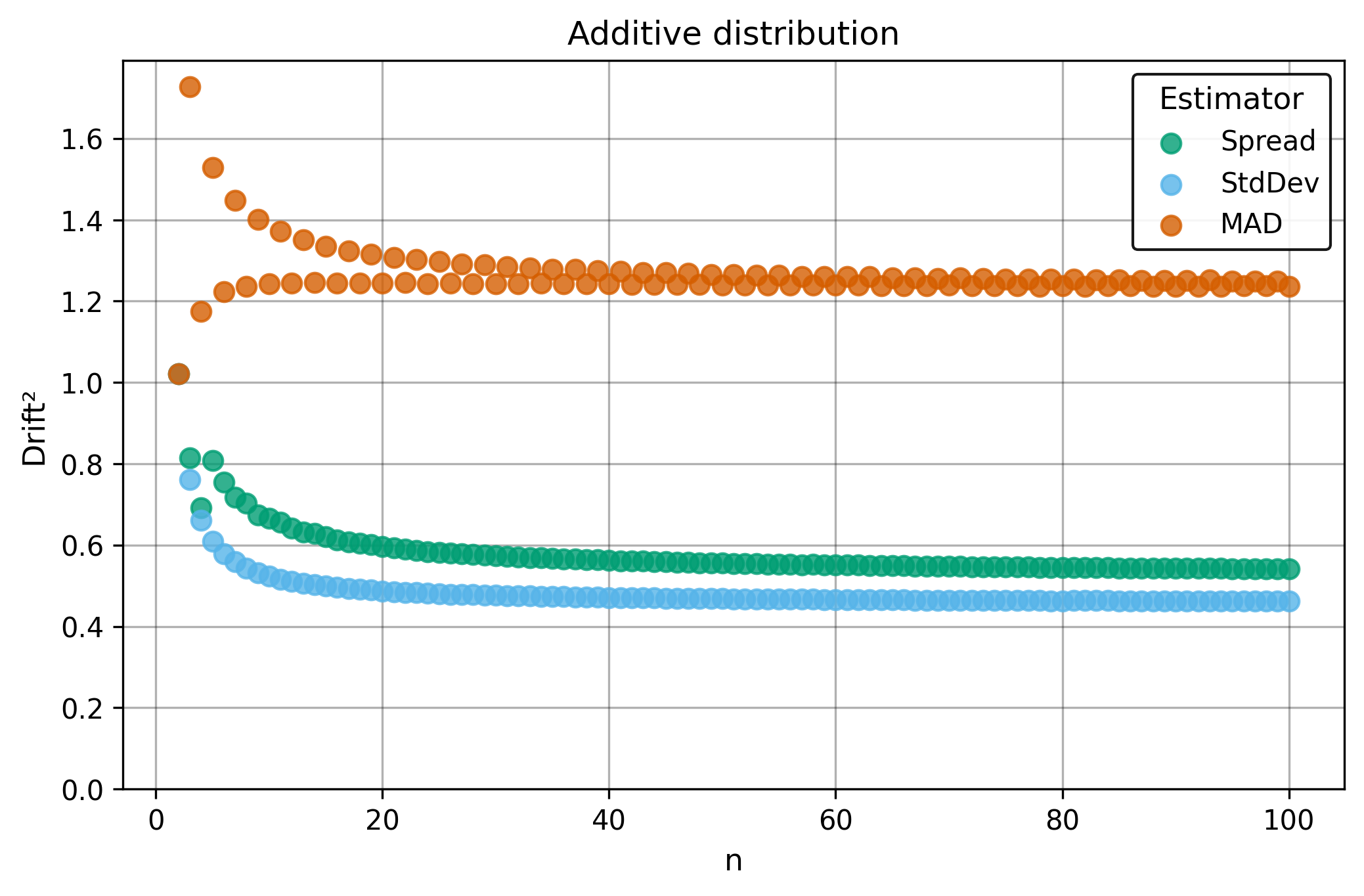
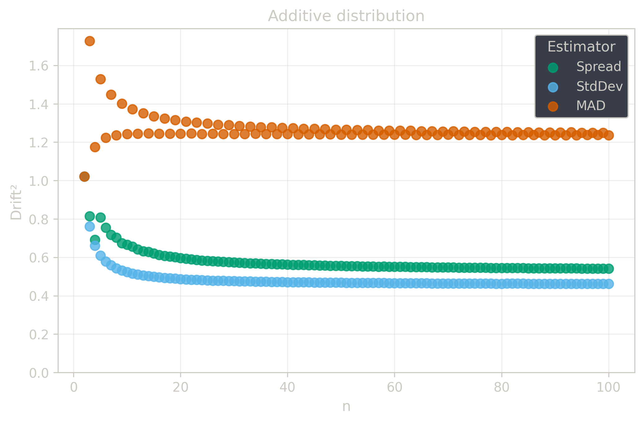
§7.1.9. Asymptotic Spread Drift
For the sample spread $\Spread(\x) = \underset{1 \leq i < j \leq n}{\Median} |x_i - x_j|$ applied to samples from $\Additive(\mathrm{mean}, \mathrm{stdDev})$, the asymptotic distribution is approximately $\Additive$ (‘Normal’).
The spread estimator computes all pairwise absolute differences and takes their median. For the $\Additive$ (‘Normal’) distribution, the population spread equals $\sqrt{2} \cdot z_{0.75} \cdot \mathrm{stdDev}$ as derived in the Asymptotic Spread Value section.
The asymptotic standard deviation of the sample spread for the $\Additive$ (‘Normal’) distribution is:
$$ \mathrm{StdDev}[\Spread(X_{1:n})] = c_{\mathrm{spr}} \cdot \frac{\mathrm{stdDev}}{\sqrt{n}} $$where $c_{\mathrm{spr}} \approx 0.72$.
Applying the lemma with $a = c_{\mathrm{spr}}$ and $b = \sqrt{2} \cdot z_{0.75}$:
$$ \Spread[\Spread(X_{1:n})] = \sqrt{2} \cdot z_{0.75} \cdot c_{\mathrm{spr}} \cdot \frac{\mathrm{stdDev}}{\sqrt{n}} $$Since $\Center[\Spread(X_{1:n})] \approx \sqrt{2} \cdot z_{0.75} \cdot \mathrm{stdDev}$ asymptotically:
$$ \RelSpread[\Spread(X_{1:n})] = \frac{\sqrt{2} \cdot z_{0.75} \cdot c_{\mathrm{spr}} \cdot \mathrm{stdDev}/\sqrt{n}}{\sqrt{2} \cdot z_{0.75} \cdot \mathrm{stdDev}} = \frac{c_{\mathrm{spr}}}{\sqrt{n}} $$Therefore:
$$ \Drift(\Spread, X) = \lim_{n \to \infty} \sqrt{n} \cdot \RelSpread[\Spread(X_{1:n})] = c_{\mathrm{spr}} $$Numerically, $c_{\mathrm{spr}} \approx 0.72$.
§7.1.10. Summary
Summary for average estimators:
| Estimator | $\Drift(E, X)$ | $\Drift^2(E, X)$ | $1/\Drift^2(E, X)$ |
|---|---|---|---|
| $\Mean$ | $1$ | $1$ | $1$ |
| $\Median$ | $\approx 1.253$ | $\pi/2 \approx 1.571$ | $2/\pi \approx 0.637$ |
| $\Center$ | $\approx 1.023$ | $\pi/3 \approx 1.047$ | $3/\pi \approx 0.955$ |
The squared drift values indicate the sample size adjustment needed when switching estimators. For instance, switching from $\Mean$ to $\Median$ while maintaining the same precision requires increasing the sample size by a factor of $\pi/2 \approx 1.571$ (about 57% more observations). Similarly, switching from $\Mean$ to $\Center$ requires only about 5% more observations.
The inverse squared drift (rightmost column) equals the classical statistical efficiency relative to the $\Mean$. The $\Mean$ achieves optimal performance (unit efficiency) for the $\Additive$ (‘Normal’) distribution, as expected from classical theory. The $\Center$ maintains 95.5% efficiency while offering greater robustness to outliers, making it an attractive alternative when some contamination is possible. The $\Median$, while most robust, operates at only 63.7% efficiency under purely $\Additive$ (‘Normal’) conditions.
Summary for dispersion estimators:
For the $\Additive$ (‘Normal’) distribution, the asymptotic drift values reveal the relative precision of different dispersion estimators:
| Estimator | $\Drift(E, X)$ | $\Drift^2(E, X)$ | $1/\Drift^2(E, X)$ |
|---|---|---|---|
| $\StdDev$ | $\approx 0.67$ | $\approx 0.45$ | $\approx 2.22$ |
| $\MAD$ | $\approx 1.10$ | $\approx 1.22$ | $\approx 0.82$ |
| $\Spread$ | $\approx 0.72$ | $\approx 0.52$ | $\approx 1.92$ |
The squared drift values indicate the sample size adjustment needed when switching estimators. For instance, switching from $\StdDev$ to $\MAD$ while maintaining the same precision requires increasing the sample size by a factor of $1.22/0.45 \approx 2.71$ (more than doubling the observations). Similarly, switching from $\StdDev$ to $\Spread$ requires a factor of $0.52/0.45 \approx 1.16$.
The $\StdDev$ achieves optimal performance for the $\Additive$ (‘Normal’) distribution. The $\MAD$ requires about 2.7 times more data to match the $\StdDev$ precision while offering greater robustness to outliers. The $\Spread$ requires about 1.16 times more data to match the $\StdDev$ precision under purely $\Additive$ (‘Normal’) conditions while maintaining robustness.
§8. Reference Implementations
§8.1. Python
Install from PyPI:
pip install pragmastat==3.2.4Source code: https://github.com/AndreyAkinshin/pragmastat/tree/v3.2.4/py
Pragmastat on PyPI: https://pypi.org/project/pragmastat/
Demo:
from pragmastat import center, spread, rel_spread, shift, ratio, avg_spread, disparity


def main():
    x = [0, 2, 4, 6, 8]
    print(center(x))  # 4
    print(center([v + 10 for v in x]))  # 14
    print(center([v * 3 for v in x]))  # 12

    print(spread(x))  # 4
    print(spread([v + 10 for v in x]))  # 4
    print(spread([v * 2 for v in x]))  # 8

    print(rel_spread(x))  # 1
    print(rel_spread([v * 5 for v in x]))  # 1

    y = [10, 12, 14, 16, 18]
    print(shift(x, y))  # -10
    print(shift(x, x))  # 0
    print(shift([v + 7 for v in x], [v + 3 for v in y]))  # -6
    print(shift([v * 2 for v in x], [v * 2 for v in y]))  # -20
    print(shift(y, x))  # 10

    x = [1, 2, 4, 8, 16]
    y = [2, 4, 8, 16, 32]
    print(ratio(x, y))  # 0.5
    print(ratio(x, x))  # 1
    print(ratio([v * 2 for v in x], [v * 5 for v in y]))  # 0.2

    x = [0, 3, 6, 9, 12]
    y = [0, 2, 4, 6, 8]
    print(spread(x))  # 6
    print(spread(y))  # 4

    print(avg_spread(x, y))  # 5
    print(avg_spread(x, x))  # 6
    print(avg_spread([v * 2 for v in x], [v * 3 for v in x]))  # 15
    print(avg_spread(y, x))  # 5
    print(avg_spread([v * 2 for v in x], [v * 2 for v in y]))  # 10

    print(shift(x, y))  # 2
    print(avg_spread(x, y))  # 5

    print(disparity(x, y))  # 0.4
    print(disparity([v + 5 for v in x], [v + 5 for v in y]))  # 0.4
    print(disparity([v * 2 for v in x], [v * 2 for v in y]))  # 0.4
    print(disparity(y, x))  # -0.4


if __name__ == "__main__":
    main()
§8.2. TypeScript
Install from npm:
npm i pragmastat@3.2.4Source code: https://github.com/AndreyAkinshin/pragmastat/tree/v3.2.4/ts
Pragmastat on npm: https://www.npmjs.com/package/pragmastat
Demo:
import { center, spread, relSpread, shift, ratio, avgSpread, disparity } from '../src';

function main() {
    let x = [0, 2, 4, 6, 8];
    console.log(center(x)); // 4
    console.log(center(x.map(v => v + 10))); // 14
    console.log(center(x.map(v => v * 3))); // 12

    console.log(spread(x)); // 4
    console.log(spread(x.map(v => v + 10))); // 4
    console.log(spread(x.map(v => v * 2))); // 8

    console.log(relSpread(x)); // 1
    console.log(relSpread(x.map(v => v * 5))); // 1

    let y = [10, 12, 14, 16, 18];
    console.log(shift(x, y)); // -10
    console.log(shift(x, x)); // 0
    console.log(shift(x.map(v => v + 7), y.map(v => v + 3))); // -6
    console.log(shift(x.map(v => v * 2), y.map(v => v * 2))); // -20
    console.log(shift(y, x)); // 10

    x = [1, 2, 4, 8, 16];
    y = [2, 4, 8, 16, 32];
    console.log(ratio(x, y)); // 0.5
    console.log(ratio(x, x)); // 1
    console.log(ratio(x.map(v => v * 2), y.map(v => v * 5))); // 0.2

    x = [0, 3, 6, 9, 12];
    y = [0, 2, 4, 6, 8];
    console.log(spread(x)); // 6
    console.log(spread(y)); // 4

    console.log(avgSpread(x, y)); // 5
    console.log(avgSpread(x, x)); // 6
    console.log(avgSpread(x.map(v => v * 2), x.map(v => v * 3))); // 15
    console.log(avgSpread(y, x)); // 5
    console.log(avgSpread(x.map(v => v * 2), y.map(v => v * 2))); // 10

    console.log(shift(x, y)); // 2
    console.log(avgSpread(x, y)); // 5

    console.log(disparity(x, y)); // 0.4
    console.log(disparity(x.map(v => v + 5), y.map(v => v + 5))); // 0.4
    console.log(disparity(x.map(v => v * 2), y.map(v => v * 2))); // 0.4
    console.log(disparity(y, x)); // -0.4
}

main();
§8.3. R
Install from GitHub:
install.packages("remotes") # If 'remotes' is not installed
remotes::install_github("AndreyAkinshin/pragmastat",
                        subdir = "r/pragmastat", ref = "v3.2.4")
library(pragmastat)
Source code: https://github.com/AndreyAkinshin/pragmastat/tree/v3.2.4/r
Demo:
library(pragmastat)

x <- c(0, 2, 4, 6, 8)
print(center(x)) # 4
print(center(x + 10)) # 14
print(center(x * 3)) # 12

print(spread(x)) # 4
print(spread(x + 10)) # 4
print(spread(x * 2)) # 8

print(rel_spread(x)) # 1
print(rel_spread(x * 5)) # 1

y <- c(10, 12, 14, 16, 18)
print(shift(x, y)) # -10
print(shift(x, x)) # 0
print(shift(x + 7, y + 3)) # -6
print(shift(x * 2, y * 2)) # -20
print(shift(y, x)) # 10

x <- c(1, 2, 4, 8, 16)
y <- c(2, 4, 8, 16, 32)
print(ratio(x, y)) # 0.5
print(ratio(x, x)) # 1
print(ratio(x * 2, y * 5)) # 0.2

x <- c(0, 3, 6, 9, 12)
y <- c(0, 2, 4, 6, 8)
print(spread(x)) # 6
print(spread(y)) # 4

print(avg_spread(x, y)) # 5
print(avg_spread(x, x)) # 6
print(avg_spread(x * 2, x * 3)) # 15
print(avg_spread(y, x)) # 5
print(avg_spread(x * 2, y * 2)) # 10

print(shift(x, y)) # 2
print(avg_spread(x, y)) # 5

print(disparity(x, y)) # 0.4
print(disparity(x + 5, y + 5)) # 0.4
print(disparity(x * 2, y * 2)) # 0.4
print(disparity(y, x)) # -0.4
§8.4. C#
Install from NuGet via .NET CLI:
dotnet add package Pragmastat --version 3.2.4Install from NuGet via Package Manager Console:
NuGet\Install-Package Pragmastat -Version 3.2.4Source code: https://github.com/AndreyAkinshin/pragmastat/tree/v3.2.4/cs
Pragmastat on NuGet: https://www.nuget.org/packages/Pragmastat/
Demo:
using static System.Console;

namespace Pragmastat.Demo;

class Program
{
  static void Main()
  {
    var x = new Sample(0, 2, 4, 6, 8);
    WriteLine(x.Center()); // 4
    WriteLine((x + 10).Center()); // 14
    WriteLine((x * 3).Center()); // 12

    WriteLine(x.Spread()); // 4
    WriteLine((x + 10).Spread()); // 4
    WriteLine((x * 2).Spread()); // 8

    WriteLine(x.RelSpread()); // 1
    WriteLine((x * 5).RelSpread()); // 1

    var y = new Sample(10, 12, 14, 16, 18);
    WriteLine(Toolkit.Shift(x, y)); // -10
    WriteLine(Toolkit.Shift(x, x)); // 0
    WriteLine(Toolkit.Shift(x + 7, y + 3)); // -6
    WriteLine(Toolkit.Shift(x * 2, y * 2)); // -20
    WriteLine(Toolkit.Shift(y, x)); // 10

    x = new Sample(1, 2, 4, 8, 16);
    y = new Sample(2, 4, 8, 16, 32);
    WriteLine(Toolkit.Ratio(x, y)); // 0.5
    WriteLine(Toolkit.Ratio(x, x)); // 1
    WriteLine(Toolkit.Ratio(x * 2, y * 5)); // 0.2

    x = new Sample(0, 3, 6, 9, 12);
    y = new Sample(0, 2, 4, 6, 8);
    WriteLine(x.Spread()); // 6
    WriteLine(y.Spread()); // 4

    WriteLine(Toolkit.AvgSpread(x, y)); // 5
    WriteLine(Toolkit.AvgSpread(x, x)); // 6
    WriteLine(Toolkit.AvgSpread(x * 2, x * 3)); // 15
    WriteLine(Toolkit.AvgSpread(y, x)); // 5
    WriteLine(Toolkit.AvgSpread(x * 2, y * 2)); // 10

    WriteLine(Toolkit.Shift(x, y)); // 2
    WriteLine(Toolkit.AvgSpread(x, y)); // 5

    WriteLine(Toolkit.Disparity(x, y)); // 0.4
    WriteLine(Toolkit.Disparity(x + 5, y + 5)); // 0.4
    WriteLine(Toolkit.Disparity(x * 2, y * 2)); // 0.4
    WriteLine(Toolkit.Disparity(y, x)); // -0.4
  }
}
§8.5. Kotlin
Install from Maven Central Repository via Apache Maven:
<dependency>
    <groupId>dev.pragmastat</groupId>
    <artifactId>pragmastat</artifactId>
    <version>3.2.4</version>
</dependency>
Install from Maven Central Repository via Gradle:
implementation 'dev.pragmastat:pragmastat:3.2.4'Install from Maven Central Repository via Gradle (Kotlin):
implementation("dev.pragmastat:pragmastat:3.2.4")Source code: https://github.com/AndreyAkinshin/pragmastat/tree/v3.2.4/kt
Pragmastat on Maven Central Repository: https://central.sonatype.com/artifact/dev.pragmastat/pragmastat/overview
Demo:
package dev.pragmastat.demo

import dev.pragmastat.*

fun main() {
    var x = listOf(0.0, 2.0, 4.0, 6.0, 8.0)
    println(center(x)) // 4
    println(center(x.map { it + 10 })) // 14
    println(center(x.map { it * 3 })) // 12

    println(spread(x)) // 4
    println(spread(x.map { it + 10 })) // 4
    println(spread(x.map { it * 2 })) // 8

    println(relSpread(x)) // 1
    println(relSpread(x.map { it * 5 })) // 1

    var y = listOf(10.0, 12.0, 14.0, 16.0, 18.0)
    println(shift(x, y)) // -10
    println(shift(x, x)) // 0
    println(shift(x.map { it + 7 }, y.map { it + 3 })) // -6
    println(shift(x.map { it * 2 }, y.map { it * 2 })) // -20
    println(shift(y, x)) // 10

    x = listOf(1.0, 2.0, 4.0, 8.0, 16.0)
    y = listOf(2.0, 4.0, 8.0, 16.0, 32.0)
    println(ratio(x, y)) // 0.5
    println(ratio(x, x)) // 1
    println(ratio(x.map { it * 2 }, y.map { it * 5 })) // 0.2

    x = listOf(0.0, 3.0, 6.0, 9.0, 12.0)
    y = listOf(0.0, 2.0, 4.0, 6.0, 8.0)
    println(spread(x)) // 6
    println(spread(y)) // 4

    println(avgSpread(x, y)) // 5
    println(avgSpread(x, x)) // 6
    println(avgSpread(x.map { it * 2 }, x.map { it * 3 })) // 15
    println(avgSpread(y, x)) // 5
    println(avgSpread(x.map { it * 2 }, y.map { it * 2 })) // 10

    println(shift(x, y)) // 2
    println(avgSpread(x, y)) // 5

    println(disparity(x, y)) // 0.4
    println(disparity(x.map { it + 5 }, y.map { it + 5 })) // 0.4
    println(disparity(x.map { it * 2 }, y.map { it * 2 })) // 0.4
    println(disparity(y, x)) // -0.4
}
§8.6. Rust
Install from crates.io via cargo:
cargo add pragmastat@3.2.4Install from crates.io via Cargo.toml:
[dependencies]
pragmastat = "3.2.4"
Source code: https://github.com/AndreyAkinshin/pragmastat/tree/v3.2.4/rs
Pragmastat on crates.io: https://crates.io/crates/pragmastat
Demo:
use pragmastat::*;

fn print(result: Result<f64, &str>) {
    println!("{}", result.unwrap());
}

fn add(x: &[f64], val: f64) -> Vec<f64> {
    x.iter().map(|v| v + val).collect()
}

fn multiply(x: &[f64], val: f64) -> Vec<f64> {
    x.iter().map(|v| v * val).collect()
}

fn main() {
    let x = vec![0.0, 2.0, 4.0, 6.0, 8.0];
    print(center(&x)); // 4
    print(center(&add(&x, 10.0))); // 14
    print(center(&multiply(&x, 3.0))); // 12

    print(spread(&x)); // 4
    print(spread(&add(&x, 10.0))); // 4
    print(spread(&multiply(&x, 2.0))); // 8

    print(rel_spread(&x)); // 1
    print(rel_spread(&multiply(&x, 5.0))); // 1

    let y = vec![10.0, 12.0, 14.0, 16.0, 18.0];
    print(shift(&x, &y)); // -10
    print(shift(&x, &x)); // 0
    print(shift(&add(&x, 7.0), &add(&y, 3.0))); // -6
    print(shift(&multiply(&x, 2.0), &multiply(&y, 2.0))); // -20
    print(shift(&y, &x)); // 10

    let x = vec![1.0, 2.0, 4.0, 8.0, 16.0];
    let y = vec![2.0, 4.0, 8.0, 16.0, 32.0];
    print(ratio(&x, &y)); // 0.5
    print(ratio(&x, &x)); // 1
    print(ratio(&multiply(&x, 2.0), &multiply(&y, 5.0))); // 0.2

    let x = vec![0.0, 3.0, 6.0, 9.0, 12.0];
    let y = vec![0.0, 2.0, 4.0, 6.0, 8.0];
    print(spread(&x)); // 6
    print(spread(&y)); // 4

    print(avg_spread(&x, &y)); // 5
    print(avg_spread(&x, &x)); // 6
    print(avg_spread(&multiply(&x, 2.0), &multiply(&x, 3.0))); // 15
    print(avg_spread(&y, &x)); // 5
    print(avg_spread(&multiply(&x, 2.0), &multiply(&y, 2.0))); // 10

    print(shift(&x, &y)); // 2
    print(avg_spread(&x, &y)); // 5

    print(disparity(&x, &y)); // 0.4
    print(disparity(&add(&x, 5.0), &add(&y, 5.0))); // 0.4
    print(disparity(&multiply(&x, 2.0), &multiply(&y, 2.0))); // 0.4
    print(disparity(&y, &x)); // -0.4
}
§8.7. Go
Install from GitHub:
go get github.com/AndreyAkinshin/pragmastat/go/v3@v3.2.4Source code: https://github.com/AndreyAkinshin/pragmastat/tree/v3.2.4/go
Demo:
package main

import (
	"fmt"
	"log"

	pragmastat "github.com/AndreyAkinshin/pragmastat/go/v3"
)

func must[T any](val T, err error) T {
	if err != nil {
		log.Fatal(err)
	}
	return val
}

func print(val float64, err error) {
	fmt.Println(must(val, err))
}

func add(x []float64, val float64) []float64 {
	result := make([]float64, len(x))
	for i, v := range x {
		result[i] = v + val
	}
	return result
}

func multiply(x []float64, val float64) []float64 {
	result := make([]float64, len(x))
	for i, v := range x {
		result[i] = v * val
	}
	return result
}

func main() {
	x := []float64{0, 2, 4, 6, 8}
	print(pragmastat.Center(x))              // 4
	print(pragmastat.Center(add(x, 10)))     // 14
	print(pragmastat.Center(multiply(x, 3))) // 12

	print(pragmastat.Spread(x))              // 4
	print(pragmastat.Spread(add(x, 10)))     // 4
	print(pragmastat.Spread(multiply(x, 2))) // 8

	print(pragmastat.RelSpread(x))              // 1
	print(pragmastat.RelSpread(multiply(x, 5))) // 1

	y := []float64{10, 12, 14, 16, 18}
	print(pragmastat.Shift(x, y))                           // -10
	print(pragmastat.Shift(x, x))                           // 0
	print(pragmastat.Shift(add(x, 7), add(y, 3)))           // -6
	print(pragmastat.Shift(multiply(x, 2), multiply(y, 2))) // -20
	print(pragmastat.Shift(y, x))                           // 10

	x = []float64{1, 2, 4, 8, 16}
	y = []float64{2, 4, 8, 16, 32}
	print(pragmastat.Ratio(x, y))                           // 0.5
	print(pragmastat.Ratio(x, x))                           // 1
	print(pragmastat.Ratio(multiply(x, 2), multiply(y, 5))) // 0.2

	x = []float64{0, 3, 6, 9, 12}
	y = []float64{0, 2, 4, 6, 8}
	print(pragmastat.Spread(x)) // 6
	print(pragmastat.Spread(y)) // 4

	print(pragmastat.AvgSpread(x, y))                           // 5
	print(pragmastat.AvgSpread(x, x))                           // 6
	print(pragmastat.AvgSpread(multiply(x, 2), multiply(x, 3))) // 15
	print(pragmastat.AvgSpread(y, x))                           // 5
	print(pragmastat.AvgSpread(multiply(x, 2), multiply(y, 2))) // 10

	print(pragmastat.Shift(x, y))     // 2
	print(pragmastat.AvgSpread(x, y)) // 5

	print(pragmastat.Disparity(x, y))                           // 0.4
	print(pragmastat.Disparity(add(x, 5), add(y, 5)))           // 0.4
	print(pragmastat.Disparity(multiply(x, 2), multiply(y, 2))) // 0.4
	print(pragmastat.Disparity(y, x))                           // -0.4
}
§9. Reference Tests
§9.1. Motivation
The toolkit maintains seven implementations across different programming languages: Python, TypeScript, R, C#, Kotlin, Rust, and Go. Each implementation must produce identical numerical results for all estimators. Maintaining correctness across this diverse set of languages requires a rigorous reference test suite.
Reference tests serve three critical purposes:
- Cross-language validation. All implementations must pass identical test cases, ensuring consistent behavior regardless of language choice.
- Regression prevention. Changes to any implementation can be validated against the reference outputs to detect unintended modifications.
- Implementation guidance. The test cases provide concrete examples that guide developers in implementing the toolkit in new languages.
The test design follows established quality assurance principles:
- Minimal sufficiency. The test set should be as small as possible while still providing high confidence in correctness. Smaller test suites reduce CI execution time and simplify maintenance.
- Comprehensive coverage. Tests must cover both typical use cases and edge cases that expose potential implementation errors.
- Deterministic reproducibility. All random test cases use fixed seeds to ensure identical results across all platforms and implementations.
The test suite balances three categories:
- Canonical cases use deterministic, easily verified inputs like natural number sequences. These provide intuitive examples where correct outputs can be validated by inspection.
- Edge cases test boundary conditions such as single-element samples, zero values, and minimum viable sample sizes. These expose off-by-one errors, division by zero, and other common implementation mistakes.
- Fuzzy tests use controlled random number generation to explore the input space beyond hand-crafted examples. Random tests catch issues that might not be apparent from simple deterministic cases.
The C# implementation serves as the reference generator. All test cases are defined programmatically, executed to produce expected outputs, and serialized to JSON. Other implementations load these JSON files and verify that their estimators produce matching results within a given numerical tolerance.
§9.2. Center Tests
$$ \Center(\x) = \underset{1 \leq i \leq j \leq n}{\Median} \left(\frac{x_i + x_j}{2} \right) $$The $\Center$ test suite contains 38 correctness test cases stored in the repository (24 original + 14 unsorted), plus 1 performance test that should be implemented manually (see §Test Framework).
Demo examples ($n = 5$) — from manual introduction, validating properties:
demo-1: $\x = (0, 2, 4, 6, 8)$, expected output: $4$ (base case)demo-2: $\x = (10, 12, 14, 16, 18)$ (= demo-1 + 10), expected output: $14$ (location equivariance)demo-3: $\x = (0, 6, 12, 18, 24)$ (= 3 × demo-1), expected output: $12$ (scale equivariance)
Natural sequences ($n = 1, 2, 3, 4$) — canonical happy path examples:
natural-1: $\x = (1)$, expected output: $1$natural-2: $\x = (1, 2)$, expected output: $1.5$natural-3: $\x = (1, 2, 3)$, expected output: $2$natural-4: $\x = (1, 2, 3, 4)$, expected output: $2.5$ (smallest even size with rich structure)
Negative values ($n = 3$) — sign handling validation:
negative-3: $\x = (-3, -2, -1)$, expected output: $-2$
Zero values ($n = 1, 2$) — edge case testing with zeros:
zeros-1: $\x = (0)$, expected output: $0$zeros-2: $\x = (0, 0)$, expected output: $0$
Additive distribution ($n = 5, 10, 30$) — fuzzy testing with $\Additive(10, 1)$:
additive-5,additive-10,additive-30: random samples generated with seed 0
Uniform distribution ($n = 5, 100$) — fuzzy testing with $\Uniform(0, 1)$:
uniform-5,uniform-100: random samples generated with seed 1
The random samples validate that $\Center$ performs correctly on realistic distributions at various sample sizes. The progression from small ($n = 5$) to large ($n = 100$) samples helps identify issues that only manifest at specific scales.
Algorithm stress tests — edge cases for fast algorithm implementation:
duplicates-5: $\x = (3, 3, 3, 3, 3)$ (all identical, stress stall handling)duplicates-10: $\x = (1, 1, 1, 2, 2, 2, 3, 3, 3, 3)$ (many duplicates, stress tie-breaking)parity-odd-7: $\x = (1, 2, 3, 4, 5, 6, 7)$ (odd sample size for odd total pairs)parity-even-6: $\x = (1, 2, 3, 4, 5, 6)$ (even sample size for even total pairs)parity-odd-49: 49-element sequence $(1, 2, \ldots, 49)$ (large odd, 1225 pairs)parity-even-50: 50-element sequence $(1, 2, \ldots, 50)$ (large even, 1275 pairs)
Extreme values — numerical stability and range tests:
extreme-large-5: $\x = (1e8, 2e8, 3e8, 4e8, 5e8)$ (very large values)extreme-small-5: $\x = (1e{-}8, 2e{-}8, 3e{-}8, 4e{-}8, 5e{-}8)$ (very small positive values)extreme-wide-5: $\x = (0.001, 1, 100, 1000, 1000000)$ (wide range, tests precision)
Unsorted tests — verify sorting correctness (14 tests):
unsorted-reverse-{n}for $n \in \{2, 3, 4, 5, 7\}$: reverse sorted natural sequences (5 tests)unsorted-shuffle-3: $\x = (2, 1, 3)$ (middle element first)unsorted-shuffle-4: $\x = (3, 1, 4, 2)$ (interleaved)unsorted-shuffle-5: $\x = (5, 2, 4, 1, 3)$ (complex shuffle)unsorted-last-first-5: $\x = (5, 1, 2, 3, 4)$ (last moved to first)unsorted-first-last-5: $\x = (2, 3, 4, 5, 1)$ (first moved to last)unsorted-duplicates-mixed-5: $\x = (3, 3, 3, 3, 3)$ (all identical, any order)unsorted-duplicates-unsorted-10: $\x = (3, 1, 2, 3, 1, 3, 2, 1, 3, 2)$ (duplicates mixed)unsorted-extreme-large-unsorted-5: $\x = (5e8, 1e8, 4e8, 2e8, 3e8)$ (large values unsorted)unsorted-parity-odd-reverse-7: $\x = (7, 6, 5, 4, 3, 2, 1)$ (odd size reverse)
These tests ensure implementations correctly sort input data before computing pairwise averages. The variety of shuffle patterns (reverse, rotation, interleaving, single element displacement) catches common sorting bugs.
Performance test — validates the fast $O(n \log n)$ algorithm:
- Input: $\x = (1, 2, 3, \ldots, 100000)$
- Expected output: $50000.5$
- Time constraint: Must complete in under 5 seconds
- Purpose: Ensures that the implementation uses the efficient algorithm rather than materializing all $\binom{n+1}{2} \approx 5$ billion pairwise averages
This test case is not stored in the repository because it generates a large JSON file (approximately 1.5 MB). Each language implementation should manually implement this test with the hardcoded expected result.
§9.3. Spread Tests
$$ \Spread(\x) = \underset{1 \leq i < j \leq n}{\Median} |x_i - x_j| $$The $\Spread$ test suite contains 38 correctness test cases stored in the repository (24 original + 14 unsorted), plus 1 performance test that should be implemented manually (see §Test Framework).
Demo examples ($n = 5$) — from manual introduction, validating properties:
demo-1: $\x = (0, 2, 4, 6, 8)$, expected output: $4$ (base case)demo-2: $\x = (10, 12, 14, 16, 18)$ (= demo-1 + 10), expected output: $4$ (location invariance)demo-3: $\x = (0, 4, 8, 12, 16)$ (= 2 × demo-1), expected output: $8$ (scale equivariance)
Natural sequences ($n = 1, 2, 3, 4$):
natural-1: $\x = (1)$, expected output: $0$ (single element has zero dispersion)natural-2: $\x = (1, 2)$, expected output: $1$natural-3: $\x = (1, 2, 3)$, expected output: $1$natural-4: $\x = (1, 2, 3, 4)$, expected output: $1.5$ (smallest even size with rich structure)
Negative values ($n = 3$) — sign handling validation:
negative-3: $\x = (-3, -2, -1)$, expected output: $1$
Zero values ($n = 1, 2$):
zeros-1: $\x = (0)$, expected output: $0$zeros-2: $\x = (0, 0)$, expected output: $0$
Additive distribution ($n = 5, 10, 30$) — $\Additive(10, 1)$:
additive-5,additive-10,additive-30: random samples generated with seed 0
Uniform distribution ($n = 5, 100$) — $\Uniform(0, 1)$:
uniform-5,uniform-100: random samples generated with seed 1
The natural sequence cases validate the basic pairwise difference calculation. The zero cases confirm that constant samples correctly produce zero spread.
Algorithm stress tests — edge cases for fast algorithm implementation:
duplicates-5: $\x = (3, 3, 3, 3, 3)$ (all identical, expected output: $0$)duplicates-10: $\x = (1, 1, 1, 2, 2, 2, 3, 3, 3, 3)$ (many duplicates, stress tie-breaking)parity-odd-7: $\x = (1, 2, 3, 4, 5, 6, 7)$ (odd sample size, 21 differences)parity-even-6: $\x = (1, 2, 3, 4, 5, 6)$ (even sample size, 15 differences)parity-odd-49: 49-element sequence $(1, 2, \ldots, 49)$ (large odd, 1176 differences)parity-even-50: 50-element sequence $(1, 2, \ldots, 50)$ (large even, 1225 differences)
Extreme values — numerical stability and range tests:
extreme-large-5: $\x = (1e8, 2e8, 3e8, 4e8, 5e8)$ (very large values)extreme-small-5: $\x = (1e{-}8, 2e{-}8, 3e{-}8, 4e{-}8, 5e{-}8)$ (very small positive values)extreme-wide-5: $\x = (0.001, 1, 100, 1000, 1000000)$ (wide range, tests precision)
Unsorted tests — verify sorting correctness (14 tests):
unsorted-reverse-{n}for $n \in \{2, 3, 4, 5, 7\}$: reverse sorted natural sequences (5 tests)unsorted-shuffle-3: $\x = (3, 1, 2)$ (rotated)unsorted-shuffle-4: $\x = (4, 2, 1, 3)$ (mixed order)unsorted-shuffle-5: $\x = (5, 1, 3, 2, 4)$ (partial shuffle)unsorted-last-first-5: $\x = (5, 1, 2, 3, 4)$ (last moved to first)unsorted-first-last-5: $\x = (2, 3, 4, 5, 1)$ (first moved to last)unsorted-duplicates-mixed-5: $\x = (3, 3, 3, 3, 3)$ (all identical)unsorted-duplicates-unsorted-10: $\x = (2, 3, 1, 3, 2, 1, 2, 3, 1, 3)$ (duplicates mixed)unsorted-extreme-wide-unsorted-5: $\x = (1000, 0.001, 1000000, 100, 1)$ (wide range unsorted)unsorted-negative-unsorted-5: $\x = (-1, -5, -2, -4, -3)$ (negative unsorted)
These tests verify that implementations correctly sort input before computing pairwise differences. Since $\Spread$ uses absolute differences, order-dependent bugs would manifest differently than in $\Center$.
Performance test — validates the fast $O(n \log n)$ algorithm:
- Input: $\x = (1, 2, 3, \ldots, 100000)$
- Expected output: $29290$
- Time constraint: Must complete in under 5 seconds
- Purpose: Ensures that the implementation uses the efficient algorithm rather than materializing all $\binom{n}{2} \approx 5$ billion pairwise differences
This test case is not stored in the repository because it generates a large JSON file (approximately 1.5 MB). Each language implementation should manually implement this test with the hardcoded expected result.
§9.4. RelSpread Tests
$$ \RelSpread(\x) = \frac{\Spread(\x)}{\left| \Center(\x) \right|} $$The $\RelSpread$ test suite contains 25 test cases (15 original + 10 unsorted) focusing on relative dispersion.
Demo examples ($n = 5$) — from manual introduction, validating properties:
demo-1: $\x = (0, 2, 4, 6, 8)$, expected output: $1$ (base case)demo-2: $\x = (0, 10, 20, 30, 40)$ (= 5 × demo-1), expected output: $1$ (scale invariance)
Natural sequences ($n = 1, 2, 3, 4$):
natural-1: $\x = (1)$, expected output: $0$natural-2: $\x = (1, 2)$, expected output: $\approx 0.667$natural-3: $\x = (1, 2, 3)$, expected output: $0.5$natural-4: $\x = (1, 2, 3, 4)$, expected output: $0.6$ (validates composite with even size)
Negative values ($n = 3$) — validates absolute value in denominator:
negative-3: $\x = (-3, -2, -1)$, expected output: $0.5$
Uniform distribution ($n = 5, 10, 20, 30, 100$) — $\Uniform(0, 1)$:
uniform-5,uniform-10,uniform-20,uniform-30,uniform-100: random samples generated with seed 0
The uniform distribution tests span multiple sample sizes to verify that $\RelSpread$ correctly normalizes dispersion. The absence of zero-value tests reflects the domain constraint requiring $\Center(\x) \neq 0$.
Composite estimator stress tests — edge cases specific to division operation:
composite-small-center: $\x = (0.001, 0.002, 0.003, 0.004, 0.005)$ (small center, tests division stability)composite-large-spread: $\x = (1, 100, 200, 300, 1000)$ (large spread relative to center)composite-extreme-ratio: $\x = (1, 1.0001, 1.0002, 1.0003, 1.0004)$ (tiny spread, tests precision)
Unsorted tests — verify sorting for composite estimator (10 tests):
unsorted-reverse-{n}for $n \in \{3, 4, 5\}$: reverse sorted natural sequences (3 tests)unsorted-shuffle-4: $\x = (4, 1, 3, 2)$ (mixed order)unsorted-shuffle-5: $\x = (5, 3, 1, 4, 2)$ (complex shuffle)unsorted-negative-unsorted-3: $\x = (-1, -3, -2)$ (negative unsorted)unsorted-demo-unsorted-5: $\x = (8, 0, 4, 2, 6)$ (demo case unsorted)unsorted-composite-small-unsorted: $\x = (0.005, 0.001, 0.003, 0.002, 0.004)$ (small center unsorted)unsorted-composite-large-unsorted: $\x = (1000, 1, 300, 100, 200)$ (large spread unsorted)unsorted-extreme-ratio-unsorted-4: $\x = (1.0003, 1, 1.0002, 1.0001)$ (extreme ratio unsorted)
Since $\RelSpread$ combines both $\Center$ and $\Spread$, these tests verify that sorting works correctly for composite estimators.
§9.5. Shift Tests
$$ \Shift(\x, \y) = \underset{1 \leq i \leq n,\,\, 1 \leq j \leq m}{\Median} \left(x_i - y_j \right) $$The $\Shift$ test suite contains 60 correctness test cases stored in the repository (42 original + 18 unsorted), plus 1 performance test that should be implemented manually (see §Test Framework).
Demo examples ($n = m = 5$) — from manual introduction, validating properties:
demo-1: $\x = (0, 2, 4, 6, 8)$, $\y = (10, 12, 14, 16, 18)$, expected output: $-10$ (base case)demo-2: $\x = (0, 2, 4, 6, 8)$, $\y = (0, 2, 4, 6, 8)$, expected output: $0$ (identity property)demo-3: $\x = (7, 9, 11, 13, 15)$, $\y = (13, 15, 17, 19, 21)$ (= demo-1 + [7,3]), expected output: $-6$ (location equivariance)demo-4: $\x = (0, 4, 8, 12, 16)$, $\y = (20, 24, 28, 32, 36)$ (= 2 × demo-1), expected output: $-20$ (scale equivariance)demo-5: $\x = (10, 12, 14, 16, 18)$, $\y = (0, 2, 4, 6, 8)$ (= reversed demo-1), expected output: $10$ (anti-symmetry)
Natural sequences ($[n, m] \in \{1, 2, 3\} \times \{1, 2, 3\}$) — 9 combinations:
natural-1-1: $\x = (1)$, $\y = (1)$, expected output: $0$natural-1-2: $\x = (1)$, $\y = (1, 2)$, expected output: $-0.5$natural-1-3: $\x = (1)$, $\y = (1, 2, 3)$, expected output: $-1$natural-2-1: $\x = (1, 2)$, $\y = (1)$, expected output: $0.5$natural-2-2: $\x = (1, 2)$, $\y = (1, 2)$, expected output: $0$natural-2-3: $\x = (1, 2)$, $\y = (1, 2, 3)$, expected output: $-0.5$natural-3-1: $\x = (1, 2, 3)$, $\y = (1)$, expected output: $1$natural-3-2: $\x = (1, 2, 3)$, $\y = (1, 2)$, expected output: $0.5$natural-3-3: $\x = (1, 2, 3)$, $\y = (1, 2, 3)$, expected output: $0$
Negative values ($[n, m] = [2, 2]$) — sign handling validation:
negative-2-2: $\x = (-2, -1)$, $\y = (-2, -1)$, expected output: $0$
Mixed-sign values ($[n, m] = [2, 2]$) — validates anti-symmetry across zero:
mixed-2-2: $\x = (-1, 1)$, $\y = (-1, 1)$, expected output: $0$
Zero values ($[n, m] \in \{1, 2\} \times \{1, 2\}$) — 4 combinations:
zeros-1-1,zeros-1-2,zeros-2-1,zeros-2-2: all produce output $0$
Additive distribution ($[n, m] \in \{5, 10, 30\} \times \{5, 10, 30\}$) — 9 combinations with $\Additive(10, 1)$:
additive-5-5,additive-5-10,additive-5-30additive-10-5,additive-10-10,additive-10-30additive-30-5,additive-30-10,additive-30-30- Random generation: $\x$ uses seed 0, $\y$ uses seed 1
Uniform distribution ($[n, m] \in \{5, 100\} \times \{5, 100\}$) — 4 combinations with $\Uniform(0, 1)$:
uniform-5-5,uniform-5-100,uniform-100-5,uniform-100-100- Random generation: $\x$ uses seed 2, $\y$ uses seed 3
The natural sequences validate anti-symmetry ($\Shift(\x, \y) = -\Shift(\y, \x)$) and the identity property ($\Shift(\x, \x) = 0$). The asymmetric size combinations test the two-sample algorithm with unbalanced inputs.
Algorithm stress tests — edge cases for fast binary search algorithm:
duplicates-5-5: $\x = (3, 3, 3, 3, 3)$, $\y = (3, 3, 3, 3, 3)$ (all identical, expected output: $0$)duplicates-10-10: $\x = (1, 1, 2, 2, 3, 3, 4, 4, 5, 5)$, $\y = (1, 1, 2, 2, 3, 3, 4, 4, 5, 5)$ (many duplicates)parity-odd-7-7: $\x = (1, 2, 3, 4, 5, 6, 7)$, $\y = (1, 2, 3, 4, 5, 6, 7)$ (odd sizes, 49 differences, expected output: $0$)parity-even-6-6: $\x = (1, 2, 3, 4, 5, 6)$, $\y = (1, 2, 3, 4, 5, 6)$ (even sizes, 36 differences, expected output: $0$)parity-asymmetric-7-6: $\x = (1, 2, 3, 4, 5, 6, 7)$, $\y = (1, 2, 3, 4, 5, 6)$ (mixed parity, 42 differences)parity-large-49-50: $\x = (1, 2, \ldots, 49)$, $\y = (1, 2, \ldots, 50)$ (large asymmetric, 2450 differences)
Extreme asymmetry — tests with very unbalanced sample sizes:
asymmetry-1-100: $\x = (50)$, $\y = (1, 2, \ldots, 100)$ (single vs many, 100 differences)asymmetry-2-50: $\x = (10, 20)$, $\y = (1, 2, \ldots, 50)$ (tiny vs medium, 100 differences)asymmetry-constant-varied: $\x = (5, 5, 5, 5, 5)$, $\y = (1, 2, 3, 4, 5, 6, 7, 8, 9, 10)$ (constant vs varied)
Unsorted tests — verify independent sorting of each sample (18 tests):
unsorted-x-natural-{n}-{m}for $(n,m) \in \{(3,3), (4,4), (5,5)\}$: X unsorted (reversed), Y sorted (3 tests)unsorted-y-natural-{n}-{m}for $(n,m) \in \{(3,3), (4,4), (5,5)\}$: X sorted, Y unsorted (reversed) (3 tests)unsorted-both-natural-{n}-{m}for $(n,m) \in \{(3,3), (4,4), (5,5)\}$: both unsorted (reversed) (3 tests)unsorted-reverse-3-3: $\x = (3, 2, 1)$, $\y = (3, 2, 1)$ (both reversed)unsorted-x-shuffle-3-3: $\x = (2, 1, 3)$, $\y = (1, 2, 3)$ (X shuffled, Y sorted)unsorted-y-shuffle-3-3: $\x = (1, 2, 3)$, $\y = (3, 1, 2)$ (X sorted, Y shuffled)unsorted-both-shuffle-4-4: $\x = (3, 1, 4, 2)$, $\y = (4, 2, 1, 3)$ (both shuffled)unsorted-duplicates-mixed-5-5: $\x = (3, 3, 3, 3, 3)$, $\y = (3, 3, 3, 3, 3)$ (all identical)unsorted-x-unsorted-duplicates: $\x = (2, 1, 3, 2, 1)$, $\y = (1, 1, 2, 2, 3)$ (X has unsorted duplicates)unsorted-y-unsorted-duplicates: $\x = (1, 1, 2, 2, 3)$, $\y = (3, 2, 1, 3, 2)$ (Y has unsorted duplicates)unsorted-asymmetric-unsorted-2-5: $\x = (2, 1)$, $\y = (5, 2, 4, 1, 3)$ (asymmetric sizes, both unsorted)unsorted-negative-unsorted-3-3: $\x = (-1, -3, -2)$, $\y = (-2, -3, -1)$ (negative unsorted)
These tests are critical for two-sample estimators because they verify that $\x$ and $\y$ are sorted independently. The variety includes cases where only one sample is unsorted, ensuring implementations don’t incorrectly assume pre-sorted input or sort samples together.
Performance test — validates the fast $O((m+n) \log L)$ binary search algorithm:
- Input: $\x = (1, 2, 3, \ldots, 100000)$, $\y = (1, 2, 3, \ldots, 100000)$
- Expected output: $0$
- Time constraint: Must complete in under 5 seconds
- Purpose: Ensures that the implementation uses the efficient algorithm rather than materializing all $mn = 10$ billion pairwise differences
This test case is not stored in the repository because it generates a large JSON file (approximately 1.5 MB). Each language implementation should manually implement this test with the hardcoded expected result.
§9.6. Ratio Tests
$$ \Ratio(\x, \y) = \underset{1 \leq i \leq n, 1 \leq j \leq m}{\Median} \left( \dfrac{x_i}{y_j} \right) $$The $\Ratio$ test suite contains 37 test cases (25 original + 12 unsorted), excluding zero values due to division constraints.
Demo examples ($n = m = 5$) — from manual introduction, validating properties:
demo-1: $\x = (1, 2, 4, 8, 16)$, $\y = (2, 4, 8, 16, 32)$, expected output: $0.5$ (base case)demo-2: $\x = (1, 2, 4, 8, 16)$, $\y = (1, 2, 4, 8, 16)$, expected output: $1$ (identity property)demo-3: $\x = (2, 4, 8, 16, 32)$, $\y = (10, 20, 40, 80, 160)$ (= [2×demo-1.x, 5×demo-1.y]), expected output: $0.2$ (scale property)
Natural sequences ($[n, m] \in \{1, 2, 3\} \times \{1, 2, 3\}$) — 9 combinations:
natural-1-1: $\x = (1)$, $\y = (1)$, expected output: $1$natural-1-2: $\x = (1)$, $\y = (1, 2)$, expected output: $\approx 0.667$natural-1-3: $\x = (1)$, $\y = (1, 2, 3)$, expected output: $0.5$natural-2-1: $\x = (1, 2)$, $\y = (1)$, expected output: $1.5$natural-2-2: $\x = (1, 2)$, $\y = (1, 2)$, expected output: $1$natural-2-3: $\x = (1, 2)$, $\y = (1, 2, 3)$, expected output: $\approx 0.833$natural-3-1: $\x = (1, 2, 3)$, $\y = (1)$, expected output: $2$natural-3-2: $\x = (1, 2, 3)$, $\y = (1, 2)$, expected output: $1.5$natural-3-3: $\x = (1, 2, 3)$, $\y = (1, 2, 3)$, expected output: $1$
Additive distribution ($[n, m] \in \{5, 10, 30\} \times \{5, 10, 30\}$) — 9 combinations with $\Additive(10, 1)$:
additive-5-5,additive-5-10,additive-5-30additive-10-5,additive-10-10,additive-10-30additive-30-5,additive-30-10,additive-30-30- Random generation: $\x$ uses seed 0, $\y$ uses seed 1
Uniform distribution ($[n, m] \in \{5, 100\} \times \{5, 100\}$) — 4 combinations with $\Uniform(0, 1)$:
uniform-5-5,uniform-5-100,uniform-100-5,uniform-100-100- Random generation: $\x$ uses seed 2, $\y$ uses seed 3
The natural sequences verify the identity property ($\Ratio(\x, \x) = 1$) and validate ratio calculations with simple integer inputs. Note that implementations should handle the practical constraint of avoiding division by values near zero.
Unsorted tests — verify independent sorting for ratio calculation (12 tests):
unsorted-x-natural-{n}-{m}for $(n,m) \in \{(3,3), (4,4)\}$: X unsorted (reversed), Y sorted (2 tests)unsorted-y-natural-{n}-{m}for $(n,m) \in \{(3,3), (4,4)\}$: X sorted, Y unsorted (reversed) (2 tests)unsorted-both-natural-{n}-{m}for $(n,m) \in \{(3,3), (4,4)\}$: both unsorted (reversed) (2 tests)unsorted-demo-unsorted-x: $\x = (16, 1, 8, 2, 4)$, $\y = (2, 4, 8, 16, 32)$ (demo-1 with X unsorted)unsorted-demo-unsorted-y: $\x = (1, 2, 4, 8, 16)$, $\y = (32, 2, 16, 4, 8)$ (demo-1 with Y unsorted)unsorted-demo-both-unsorted: $\x = (8, 1, 16, 4, 2)$, $\y = (16, 32, 2, 8, 4)$ (demo-1 both unsorted)unsorted-identity-unsorted: $\x = (4, 1, 8, 2, 16)$, $\y = (16, 1, 8, 4, 2)$ (identity property, both unsorted)unsorted-asymmetric-unsorted-2-3: $\x = (2, 1)$, $\y = (3, 1, 2)$ (asymmetric, both unsorted)unsorted-power-unsorted-5: $\x = (16, 2, 8, 1, 4)$, $\y = (32, 4, 16, 2, 8)$ (powers of 2 unsorted)
§9.7. AvgSpread Tests
$$ \AvgSpread(\x, \y) = \dfrac{n\Spread(\x) + m\Spread(\y)}{n + m} $$The $\AvgSpread$ test suite contains 49 test cases (35 original + 14 unsorted). Since $\AvgSpread$ computes $\Spread(\x)$ and $\Spread(\y)$ independently, unsorted tests are critical to verify that both samples are sorted independently before computing their spreads.
Demo examples ($n = m = 5$) — from manual introduction, validating properties:
demo-1: $\x = (0, 3, 6, 9, 12)$, $\y = (0, 2, 4, 6, 8)$, expected output: $5$ (base case: $(5 \cdot 6 + 5 \cdot 4)/10$)demo-2: $\x = (0, 3, 6, 9, 12)$, $\y = (0, 3, 6, 9, 12)$, expected output: $6$ (identity case)demo-3: $\x = (0, 6, 12, 18, 24)$, $\y = (0, 9, 18, 27, 36)$ (= [2×demo-1.x, 3×demo-1.y]), expected output: $15$ (scale equivariance)demo-4: $\x = (0, 2, 4, 6, 8)$, $\y = (0, 3, 6, 9, 12)$ (= reversed demo-1), expected output: $5$ (symmetry)demo-5: $\x = (0, 6, 12, 18, 24)$, $\y = (0, 4, 8, 12, 16)$ (= 2 × demo-1), expected output: $10$ (uniform scaling)
Natural sequences ($[n, m] \in \{1, 2, 3\} \times \{1, 2, 3\}$) — 9 combinations:
- All combinations from single-element to three-element samples, validating the weighted average calculation
Negative values ($[n, m] = [2, 2]$) — validates spread calculation with negative values:
negative-2-2: $\x = (-2, -1)$, $\y = (-2, -1)$, expected output: $1$
Zero values ($[n, m] \in \{1, 2\} \times \{1, 2\}$) — 4 combinations:
- All produce output $0$ since $\Spread$ of constant samples is zero
Additive distribution ($[n, m] \in \{5, 10, 30\} \times \{5, 10, 30\}$) — 9 combinations with $\Additive(10, 1)$:
- Tests pooled dispersion across different sample size combinations
- Random generation: $\x$ uses seed 0, $\y$ uses seed 1
Uniform distribution ($[n, m] \in \{5, 100\} \times \{5, 100\}$) — 4 combinations with $\Uniform(0, 1)$:
- Validates correct weighting when sample sizes differ substantially
- Random generation: $\x$ uses seed 2, $\y$ uses seed 3
The asymmetric size combinations are particularly important for $\AvgSpread$ because the estimator must correctly weight each sample’s contribution by its size.
Composite estimator stress tests — edge cases for weighted averaging:
composite-asymmetric-weights: $\x = (1, 2)$, $\y = (3, 4, 5, 6, 7, 8, 9, 10)$ (2 vs 8, tests weighting formula)composite-zero-spread-one: $\x = (5, 5, 5)$, $\y = (1, 2, 3, 4, 5)$ (one zero spread, tests edge case)composite-extreme-sizes: $\x = (10)$, $\y = (1, 2, 3, 4, 5, 6, 7, 8, 9, 10)$ (1 vs 10, extreme weighting)
Unsorted tests — critical for verifying independent sorting (14 tests):
unsorted-x-natural-{n}-{m}for $(n,m) \in \{(3,3), (4,4)\}$: X unsorted (reversed), Y sorted (2 tests)unsorted-y-natural-{n}-{m}for $(n,m) \in \{(3,3), (4,4)\}$: X sorted, Y unsorted (reversed) (2 tests)unsorted-both-natural-{n}-{m}for $(n,m) \in \{(3,3), (4,4)\}$: both unsorted (reversed) (2 tests)unsorted-demo-unsorted-x: $\x = (12, 0, 6, 3, 9)$, $\y = (0, 2, 4, 6, 8)$ (demo-1 with X unsorted)unsorted-demo-unsorted-y: $\x = (0, 3, 6, 9, 12)$, $\y = (8, 0, 4, 2, 6)$ (demo-1 with Y unsorted)unsorted-demo-both-unsorted: $\x = (9, 0, 12, 3, 6)$, $\y = (6, 0, 8, 2, 4)$ (demo-1 both unsorted)unsorted-identity-unsorted: $\x = (6, 0, 12, 3, 9)$, $\y = (9, 0, 12, 6, 3)$ (demo-2 unsorted)unsorted-negative-unsorted: $\x = (-1, -2)$, $\y = (-1, -2)$ (negative unsorted)unsorted-zero-unsorted-2-2: $\x = (0, 0)$, $\y = (0, 0)$ (zeros, any order)unsorted-asymmetric-weights-unsorted: $\x = (2, 1)$, $\y = (8, 3, 6, 4, 10, 5, 9, 7)$ (asymmetric unsorted)unsorted-zero-spread-x-unsorted: $\x = (5, 5, 5)$, $\y = (5, 1, 4, 2, 3)$ (zero spread X, Y unsorted)
These tests verify that implementations compute $\Spread(\x)$ and $\Spread(\y)$ with properly sorted samples.
§9.8. Disparity Tests
$$ \Disparity(\x, \y) = \dfrac{\Shift(\x, \y)}{\AvgSpread(\x, \y)} $$The $\Disparity$ test suite contains 28 test cases (16 original + 12 unsorted). Since $\Disparity$ combines $\Shift$ and $\AvgSpread$, unsorted tests verify both components handle sorting correctly.
Demo examples ($n = m = 5$) — from manual introduction, validating properties:
demo-1: $\x = (0, 3, 6, 9, 12)$, $\y = (0, 2, 4, 6, 8)$, expected output: $0.4$ (base case: $2/5$)demo-2: $\x = (5, 8, 11, 14, 17)$, $\y = (5, 7, 9, 11, 13)$ (= demo-1 + 5), expected output: $0.4$ (location invariance)demo-3: $\x = (0, 6, 12, 18, 24)$, $\y = (0, 4, 8, 12, 16)$ (= 2 × demo-1), expected output: $0.4$ (scale invariance)demo-4: $\x = (0, 2, 4, 6, 8)$, $\y = (0, 3, 6, 9, 12)$ (= reversed demo-1), expected output: $-0.4$ (anti-symmetry)
Natural sequences ($[n, m] \in \{2, 3\} \times \{2, 3\}$) — 4 combinations:
natural-2-2,natural-2-3,natural-3-2,natural-3-3- Minimum size $n, m \geq 2$ required for meaningful dispersion calculations
Negative values ($[n, m] = [2, 2]$) — end-to-end validation with negative values:
negative-2-2: $\x = (-2, -1)$, $\y = (-2, -1)$, expected output: $0$
Uniform distribution ($[n, m] \in \{5, 100\} \times \{5, 100\}$) — 4 combinations with $\Uniform(0, 1)$:
uniform-5-5,uniform-5-100,uniform-100-5,uniform-100-100- Random generation: $\x$ uses seed 0, $\y$ uses seed 1
The smaller test set for $\Disparity$ reflects implementation confidence. Since $\Disparity$ combines $\Shift$ and $\AvgSpread$, correct implementation of those components ensures $\Disparity$ correctness. The test cases validate the division operation and confirm scale-free properties.
Composite estimator stress tests — edge cases for effect size calculation:
composite-small-avgspread: $\x = (10.001, 10.002, 10.003)$, $\y = (10.004, 10.005, 10.006)$ (tiny spread, large shift)composite-large-avgspread: $\x = (1, 100, 200)$, $\y = (50, 150, 250)$ (large spread, small shift)composite-extreme-disparity: $\x = (1, 1.001)$, $\y = (100, 100.001)$ (extreme ratio, tests precision)
Unsorted tests — verify both Shift and AvgSpread handle sorting (12 tests):
unsorted-x-natural-{n}-{m}for $(n,m) \in \{(3,3), (4,4)\}$: X unsorted (reversed), Y sorted (2 tests)unsorted-y-natural-{n}-{m}for $(n,m) \in \{(3,3), (4,4)\}$: X sorted, Y unsorted (reversed) (2 tests)unsorted-both-natural-{n}-{m}for $(n,m) \in \{(3,3), (4,4)\}$: both unsorted (reversed) (2 tests)unsorted-demo-unsorted-x: $\x = (12, 0, 6, 3, 9)$, $\y = (0, 2, 4, 6, 8)$ (demo-1 with X unsorted)unsorted-demo-unsorted-y: $\x = (0, 3, 6, 9, 12)$, $\y = (8, 0, 4, 2, 6)$ (demo-1 with Y unsorted)unsorted-demo-both-unsorted: $\x = (9, 0, 12, 3, 6)$, $\y = (6, 0, 8, 2, 4)$ (demo-1 both unsorted)unsorted-location-invariance-unsorted: $\x = (17, 5, 11, 8, 14)$, $\y = (13, 5, 9, 7, 11)$ (demo-2 unsorted)unsorted-scale-invariance-unsorted: $\x = (24, 0, 12, 6, 18)$, $\y = (16, 0, 8, 4, 12)$ (demo-3 unsorted)unsorted-anti-symmetry-unsorted: $\x = (8, 0, 4, 2, 6)$, $\y = (12, 0, 6, 3, 9)$ (demo-4 reversed and unsorted)
As a composite estimator, $\Disparity$ tests both the numerator ($\Shift$) and denominator ($\AvgSpread$). Unsorted variants verify end-to-end correctness including invariance properties.
§9.9. Test Framework
The reference test framework consists of three components:
Test generation — The C# implementation defines test inputs programmatically using builder patterns.
For deterministic cases, inputs are explicitly specified.
For random cases, the framework uses controlled seeds with System.Random to ensure reproducibility across all platforms.
The random generation mechanism works as follows:
- Each test suite builder maintains a seed counter initialized to zero.
- For one-sample estimators, each distribution type receives the next available seed. The same random generator produces all samples for all sizes within that distribution.
- For two-sample estimators, each pair of distributions receives two consecutive seeds: one for the $\x$ sample generator and one for the $\y$ sample generator.
- The seed counter increments with each random generator creation, ensuring deterministic test data generation.
For $\Additive$ distributions, random values are generated using the Box-Müller transform, which converts pairs of uniform random values into normally distributed values. The transform applies the formula:
$$ X = \mu + \sigma \sqrt{-2 \ln(U_1)} \sin(2\pi U_2) $$where $U_1, U_2$ are uniform random values from $\Uniform(0, 1)$, $\mu$ is the mean, and $\sigma$ is the standard deviation.
For $\Uniform$ distributions, random values are generated directly using the quantile function:
$$ X = \min + U \cdot (\max - \min) $$where $U$ is a uniform random value from $\Uniform(0, 1)$.
The framework executes the reference implementation on all generated inputs and serializes input-output pairs to JSON format.
Test validation — Each language implementation loads the JSON test cases and executes them against its local estimator implementation. Assertions verify that outputs match expected values within a given numerical tolerance (typically $10^{-10}$ for relative error).
Test data format — Each test case is a JSON file containing input and output fields.
For one-sample estimators, the input contains array x and optional parameters.
For two-sample estimators, input contains arrays x and y.
Output is a single numeric value.
Performance testing — The toolkit provides $O(n \log n)$ fast algorithms for $\Center$, $\Spread$, and $\Shift$ estimators, dramatically more efficient than naive implementations that materialize all pairwise combinations. Performance tests use sample size $n = 100{,}000$ (for one-sample) or $n = m = 100{,}000$ (for two-sample). This specific size creates a clear performance distinction: fast implementations ($O(n \log n)$ or $O((m+n) \log L)$) complete in under 5 seconds on modern hardware across all supported languages, while naive implementations ($O(n^2 \log n)$ or $O(mn \log(mn))$) would be prohibitively slow (taking hours or failing due to memory exhaustion). With $n = 100{,}000$, naive approaches would need to materialize approximately 5 billion pairwise values for $\Center$/$\Spread$ or 10 billion for $\Shift$, whereas fast algorithms require only $O(n)$ additional memory. Performance tests serve dual purposes: correctness validation at scale and performance regression detection, ensuring implementations use the efficient algorithms and remain practical for real-world datasets with hundreds of thousands of observations. Performance test specifications are provided in the respective estimator sections above.
This framework ensures that all seven language implementations maintain strict numerical agreement across the full test suite.
§10. Artifacts
Manual:
- PDF: pragmastat-v3.2.4.pdf
- Markdown: pragmastat-v3.2.4.md
- Website: web-v3.2.4.zip
Implementations:
- Python: py-v3.2.4.zip
- TypeScript: ts-v3.2.4.zip
- R: r-v3.2.4.zip
- C#: cs-v3.2.4.zip
- Kotlin: kt-v3.2.4.zip
- Rust: rs-v3.2.4.zip
- Go: go-v3.2.4.zip
Data:
- Reference tests (json): tests-v3.2.4.zip
- Reference simulations (json): sim-v3.2.4.zip
Source code: